Finance Applications Using Geometric Sequences and Recurrence Relations Revision Notes for VCE SSCE General Mathematics

Finance Applications Using Geometric Sequences and Recurrence Relations

Introduction to geometric growth and decay

Geometric growth and geometric decay occur when a quantity increases or decreases by the same percentage at regular intervals. This type of pattern appears frequently in real-world financial situations.

Common examples include:

Compound interest on investments or loans
Reducing-balance depreciation on vehicles and equipment

infoNote

In reducing-balance depreciation, an asset loses value by a constant percentage of its current (depreciated) value each year, rather than by a fixed dollar amount. This creates a geometric decay pattern because the percentage is applied to the remaining value, not the original value.

Understanding recurrence models for growth and decay

A recurrence relation for a geometric sequence consists of two parts:

A starting value (initial term)
A rule to generate the next term from the current term

The general form is: $V_0 = \text{starting value}$ , $V_{n+1} = R \times V_n$

Identifying growth versus decay

The value of $R$ determines whether the sequence grows or decays:

chatImportant

Critical distinction:

For geometric growth: $V_{n+1} = RV_n$ $V_{n + 1} = R V_{n}$ where R > 1
- Example: $V_0 = 10$ , $V_{n+1} = 5V_n$ (grows by multiplying by 5)
For geometric decay: $V_{n+1} = RV_n$ $V_{n + 1} = R V_{n}$ where 0 < R < 1
- Example: $V_0 = 10$ , $V_{n+1} = 0.5V_n$ (decays by multiplying by 0.5)

Key insight: When $R > 1$ , each term is larger than the previous term, creating growth. When $0 < R < 1$ , each term is smaller than the previous term, creating decay.

Compound interest investments and loans

While simple interest is sometimes used, compound interest is far more common in real financial situations. With compound interest, any interest earned in one period is added to the principal and then earns interest itself in the next period.

This creates a snowball effect where the amount of interest earned increases over time. The investment value grows geometrically.

The recurrence relation for compound interest

For compound interest investments and loans (compounding yearly):

Let $V_n$ be the value of the investment after $n$ years.

Let $r$ be the percentage interest rate per compound period.

The recurrence relation is:

$V_0 = \text{principal}, \quad V_{n+1} = R \times V_n$

where:

$R = 1 + \frac{r}{100}$

infoNote

Why this formula works: If interest is 5% per annum, the value increases by 5% each year. This means the new value is 100% + 5% = 105% of the old value, which is the same as multiplying by 1.05.

Notice the plus sign in the formula - we're adding the interest rate because the value is growing.

Worked example: calculating investment growth

lightbulbExample

Worked Example: Investment Growth with Compound Interest

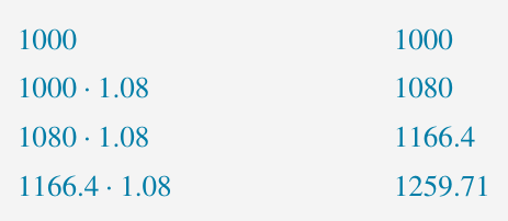
Problem: An investment of $1000 pays 8% interest per annum, compounding yearly. The recurrence relation is:

$V_0 = 1000, \quad V_{n+1} = 1.08V_n$

where $V_n$ is the value after $n$ years.

Part a: Find the value after 1, 2, and 3 years.

Solution:

Starting with $V_0 = 1000$ , we apply the recurrence relation repeatedly:

$V_0 = 1000$

$V_1 = 1.08 \times V_0 = 1.08 \times 1000 = \$1080$

$V_2 = 1.08 \times V_1 = 1.08 \times 1080 = \$1166.40$

$V_3 = 1.08 \times V_2 = 1.08 \times 1166.40 = \$1259.71$

Using a calculator, you can generate these values efficiently:

Table

Part b: When will the investment first exceed $1500?

Solution:

Continue applying the recurrence relation and count how many times you multiply by 1.08 until the value exceeds $1500.

Answer: The investment will first exceed $1500 after 6 years.

chatImportant

Exam tip: Use your CAS calculator to apply the recurrence relation repeatedly. Count the number of steps carefully to determine how many compounding periods have passed.

Different compounding periods

Interest can compound at different frequencies: yearly, quarterly, or monthly. You must adjust your recurrence relation accordingly.

lightbulbExample

Worked Example: Different Compounding Periods

Sally borrows $6000 from a bank at 4.2% per annum. Write the recurrence relation if interest compounds:

a) Yearly compounding

Let $V_n$ be the value of Sally's loan after $n$ years.

The interest rate is 4.2% per annum, so:

$R = 1 + \frac{4.2}{100} = 1.042$

Recurrence relation: $V_0 = 6000$ , $V_{n+1} = 1.042 \times V_n$

b) Quarterly compounding

Let $V_n$ be the value of Sally's loan after $n$ quarters.

Since interest is 4.2% per annum, the quarterly rate is:

$\frac{4.2}{4} = 1.05\% \text{ per quarter}$

$R = 1 + \frac{1.05}{100} = 1.0105$

Recurrence relation: $V_0 = 6000$ , $V_{n+1} = 1.0105 \times V_n$

c) Monthly compounding

Let $V_n$ be the value of Sally's loan after $n$ months.

Since interest is 4.2% per annum, the monthly rate is:

$\frac{4.2}{12} = 0.35\% \text{ per month}$

$R = 1 + \frac{0.35}{100} = 1.0035$

Recurrence relation: $V_0 = 6000$ , $V_{n+1} = 1.0035 \times V_n$

infoNote

Key principle: Divide the annual interest rate by the number of compounding periods per year (4 for quarterly, 12 for monthly) before calculating $R$ .

Reducing-balance depreciation

Reducing-balance depreciation is a method where an asset's value decreases by a constant percentage of its current value each year. Unlike flat-rate depreciation (which subtracts a fixed amount), reducing-balance depreciation results in geometric decay.

The calculations mirror compound interest, but with decay rather than growth.

The recurrence relation for reducing-balance depreciation

Let $V_n$ be the value of the asset after $n$ years.

Let $r$ be the annual percentage depreciation.

The recurrence relation is:

$V_0 = \text{initial value}, \quad V_{n+1} = R \times V_n$

where:

$R = 1 - \frac{r}{100}$

infoNote

Why this formula works: If depreciation is 10% per year, the asset retains 100% - 10% = 90% of its value, which is the same as multiplying by 0.9.

Notice the minus sign in the formula - we're subtracting the depreciation rate because the value is decreasing.

Worked example: calculating depreciation

lightbulbExample

Worked Example: Calculating Reducing-Balance Depreciation

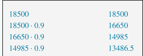
Problem: A car is purchased for $18,500. It depreciates by 10% of its value each year. The recurrence relation is:

$V_0 = 18500, \quad V_{n+1} = 0.9 \times V_n$

where $V_n$ is the car's value after $n$ years.

Part a: Find the car's value after 1, 2, and 3 years.

Solution:

The recurrence relation tells us: "to find the next value, multiply the current value by 0.9."

Starting with $V_0 = 18500$ :

$V_0 = 18500$

$V_1 = 0.9 \times V_0 = 0.9 \times 18500 = \$16650$

$V_2 = 0.9 \times V_1 = 0.9 \times 16650 = \$14985$

$V_3 = 0.9 \times V_2 = 0.9 \times 14985 = \$13486.50$

Using a calculator:

Table

Part b: When will the car first be worth less than $10,000?

Solution:

Continue applying the recurrence relation and count the number of decreases until the value falls below $10,000:

Table

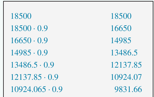
Answer: The car's value will first be less than $10,000 after 6 years.

chatImportant

Exam tip: For both compound interest and depreciation problems, use your calculator to iterate the recurrence relation. Keep careful count of the number of periods that have passed.

Section summary

bookmarkSummary

Geometric growth and decay:

$V_{n+1} = RV_n$ for R > 1 generates geometric growth
$V_{n+1} = RV_n$ for 0 < R < 1 generates geometric decay

Compound interest formula:

Let $V_n$ be the value after $n$ years and $r$ be the percentage interest per compound period.

$V_0 = \text{principal}, \quad V_{n+1} = R \times V_n, \quad \text{where } R = 1 + \frac{r}{100}$

Reducing-balance depreciation formula:

Let $V_n$ be the value after $n$ years and $r$ be the annual percentage depreciation.

$V_0 = \text{initial value}, \quad V_{n+1} = R \times V_n, \quad \text{where } R = 1 - \frac{r}{100}$

For different compounding periods: Divide the annual interest rate by the number of periods per year before calculating $R$ .

Remember!

bookmarkSummary

Key Points to Remember:

Geometric growth happens when R > 1. This models compound interest on investments and loans. Each term is larger than the previous term.
Geometric decay happens when 0 < R < 1. This models reducing-balance depreciation. Each term is smaller than the previous term.
For compound interest, use $R = 1 + \frac{r}{100}$ (add the percentage because value increases). For quarterly compounding, divide the annual rate by 4. For monthly, divide by 12.
For reducing-balance depreciation, use $R = 1 - \frac{r}{100}$ (subtract the percentage because value decreases).
Use your CAS calculator efficiently to apply recurrence relations repeatedly. Count iterations carefully to determine when a threshold is reached.

Finance Applications Using Geometric Sequences and Recurrence Relations (VCE SSCE General Mathematics): Revision Notes