The Graph, Expectation, and Variance of a Binomial Distribution Revision Notes for VCE SSCE Mathematical Methods

The Graph, Expectation, and Variance of a Binomial Distribution

Introduction

infoNote

Building on our understanding of discrete probability distributions, we now explore specific properties of the binomial distribution. This section focuses on two key aspects:

Visualizing binomial distributions through graphs
Calculating expectation and variance using efficient formulas

The graph of a binomial probability distribution

A probability distribution can be represented in several ways: as a rule, a table, or a graph. Let's investigate how the shape of a binomial probability distribution graph changes with different values of the parameters $n$ (number of trials) and $p$ (probability of success).

How the value of p affects the graph shape

chatImportant

The probability of success, $p$ , has a significant impact on the shape of the distribution:

When $p < 0.5$ : The graph is positively skewed (skewed to the right). Most of the probability is concentrated on the lower values, with a tail extending towards higher values.
When $p = 0.5$ : The graph is symmetrical. The probability of success equals the probability of failure, creating a balanced distribution.
When $p > 0.5$ : The graph is negatively skewed (skewed to the left). Most of the probability is concentrated on the higher values, with a tail extending towards lower values.

lightbulbExample

Worked Example: Comparing distributions for different p values

Construct and compare the graph of the binomial probability distribution for 20 trials ( $n = 20$ ) with probability of success:

a) $p = 0.2$

b) $p = 0.5$

c) $p = 0.8$

Solution:

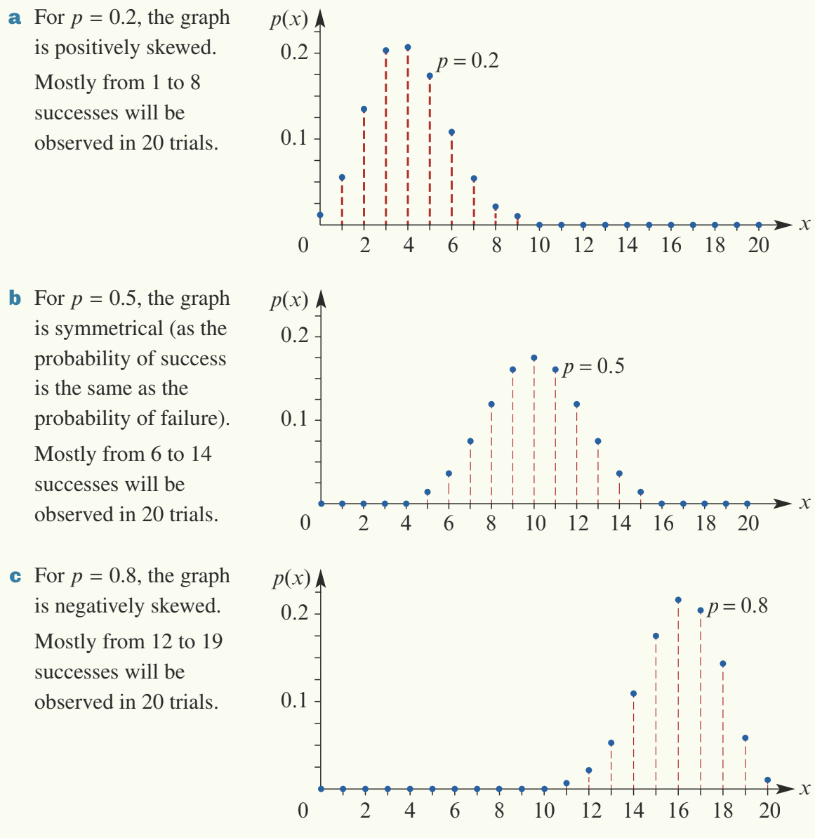
a) For $p = 0.2$ , the graph is positively skewed.

The distribution shows that mostly between 1 and 8 successes will be observed in 20 trials. The highest probabilities occur for lower numbers of successes, which makes sense because with only a 20% chance of success on each trial, we expect fewer total successes.

b) For $p = 0.5$ , the graph is symmetrical.

The probability of success is the same as the probability of failure, creating a balanced distribution. Mostly between 6 and 14 successes will be observed in 20 trials. The distribution peaks at 10 successes, which is exactly half of the 20 trials.

c) For $p = 0.8$ , the graph is negatively skewed.

With an 80% chance of success on each trial, mostly between 12 and 19 successes will be observed in 20 trials. The distribution is concentrated towards higher numbers of successes.

Key observation: Notice that the graphs for $p = 0.2$ and $p = 0.8$ are mirror images of each other. This symmetry makes sense because succeeding 80% of the time is the opposite of succeeding only 20% of the time.

Expectation and variance

Understanding expectation intuitively

infoNote

Consider this question: How many heads would you expect to obtain, on average, if a fair coin was tossed 10 times?

While the exact number of heads would vary from trial to trial (and could theoretically be anywhere from 0 to 10), intuition suggests that the long-run average would be 5 heads. This intuition is correct! For a binomial random variable $X$ with $n = 10$ and $p = 0.5$ :

E(X) = \sum_{x} x \cdot \Pr(X = x) = 5

Formulas for expectation and variance

For any binomial distribution, we can calculate the expected value and variance directly from the parameters $n$ and $p$ , without needing to work through the full probability distribution.

chatImportant

If $X$ is the number of successes in $n$ trials, each with probability of success $p$ , then:

E(X) = np

\text{Var}(X) = np(1 - p)

These formulas provide a quick and efficient way to find the centre and spread of a binomial distribution.

infoNote

The term $(1 - p)$ represents the probability of failure, often denoted as $q$ . So the variance formula can also be written as $\text{Var}(X) = npq$ .

lightbulbExample

Worked Example: Multiple-choice test

An examination consists of 30 multiple-choice questions, each question having three possible answers. A student guesses the answer to every question. Let $X$ be the number of correct answers.

a) How many will she expect to get correct? That is, find $E(X) = \mu$ .

b) Find $\text{Var}(X)$ .

Solution:

The number of correct answers, $X$ , is a binomial random variable with parameters $n = 30$ and $p = \frac{1}{3}$ (since there are three possible answers and only one is correct).

a) Using the formula for expectation:

\mu = E(X) = np

The student has an expected result of $\mu = 10$ correct answers.

Note: This is not enough to pass if the pass mark is 50% (which would require 15 correct answers).

b) Using the formula for variance:

\text{Var}(X) = np(1 - p)

\approx 6.67

lightbulbExample

Worked Example: Influenza spread with standard deviation

The probability of contracting influenza this winter is known to be 0.2. Of the 100 employees at a certain business, how many would the owner expect to get influenza? Find the standard deviation of the number who will get influenza and calculate $\mu \pm 2\sigma$ . Interpret the interval $[\mu - 2\sigma, \mu + 2\sigma]$ for this example.

Solution:

The number of employees who get influenza is a binomial random variable, $X$ , with parameters $n = 100$ and $p = 0.2$ .

Finding the expectation:

\mu = E(X) = np

The owner will expect 20 of the employees to contract influenza.

Finding the variance and standard deviation:

\sigma^2 = \text{Var}(X) = np(1 - p)

Therefore, the standard deviation is:

\sigma = \sqrt{16} = 4

Calculating the interval:

\mu \pm 2\sigma = 20 \pm (2 \times 4)

This gives us the interval [12, 28].

Interpretation:

The owner of the business knows there is a probability of approximately 0.95 (or 95%) that between 12 and 28 of the employees will contract influenza this winter.

This interpretation uses the empirical rule (also called the 68-95-99.7 rule), which states that for many distributions, approximately 95% of values fall within two standard deviations of the mean.

Exam tips

infoNote

Essential Tips for Success:

Always identify the parameters $n$ and $p$ clearly before calculating expectation or variance.
Remember that $(1 - p)$ represents the probability of failure.
The expectation $E(X) = np$ gives the long-run average, not a guarantee of what will happen in any single set of trials.
The interval $\mu \pm 2\sigma$ captures approximately 95% of possible outcomes, making it useful for predicting reasonable ranges.
When the question asks for standard deviation, don't forget to take the square root of the variance!

bookmarkSummary

Key Points to Remember:

Graph shapes depend on $p$ : Positively skewed when $p < 0.5$ , symmetrical when $p = 0.5$ , and negatively skewed when $p > 0.5$ .
Expectation formula: $E(X) = np$ gives the expected number of successes in $n$ trials.
Variance formula: $\text{Var}(X) = np(1-p)$ measures how spread out the distribution is.
Standard deviation: Remember to take the square root of variance to find $\sigma = \sqrt{np(1-p)}$ .
The $\mu \pm 2\sigma$ interval: Contains approximately 95% of all possible outcomes, providing a useful range for predictions.

The Graph, Expectation, and Variance of a Binomial Distribution (VCE SSCE Mathematical Methods): Revision Notes