Dijkstra’s Shortest Path Algorithm Revision Notes for AQA A-Level Computer Science

Dijkstra's Shortest Path Algorithm

Introduction to Dijkstra's algorithm

Dijkstra's shortest path algorithm is a fundamental computer science method for finding the most efficient route between points in a network. Named after Dutch computer scientist Edsger Dijkstra, who introduced it in 1959, this algorithm solves a common problem: how do you find the quickest or cheapest path from one location to another when you have multiple possible routes?

The algorithm works with a special data structure called a graph, which you studied in Chapter 10. It calculates the shortest distance between two points (called vertices or nodes) by considering all possible paths and systematically selecting the most efficient one. What makes this algorithm particularly useful is that it doesn't just find the shortest path to one destination – it actually calculates the shortest path from your starting point to every other point in the network.

infoNote

Dijkstra's algorithm is particularly powerful because it solves multiple problems at once: while finding the shortest path to a specific destination, it also calculates the shortest paths to all other vertices in the network from your starting point. This makes it extremely efficient for navigation and routing applications.

For example, imagine you need to find the shortest driving distance between Town A and Town E. You could try every possible route and compare them, but this becomes impractical when you have many towns and connections. That's where Dijkstra's algorithm becomes invaluable.

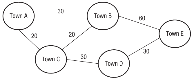
The diagram above shows a simple network of five towns with the distances between them marked on each connection. Using trial and error, you could work out all possible routes:

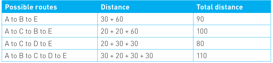
As you can see from this table, the shortest route from A to E is 80 units (going A → C → D → E). However, with more complex networks containing dozens or hundreds of points, this manual approach becomes impossible. Dijkstra's algorithm provides a systematic and efficient method to solve this problem.

Understanding graphs and key concepts

Before exploring how Dijkstra's algorithm works, let's review some important concepts about graphs:

Graph structure: Graphs are made up of two main components:

Vertices (also called nodes): These are the points or locations in your network
Edges: These are the connections or paths between vertices

Weighted graphs: In Dijkstra's algorithm, we work with weighted graphs, where each edge has a numerical value attached to it. This value might represent distance, time, cost, or any other metric you want to optimise. The algorithm only works correctly with positive weights on the edges.

chatImportant

Critical Limitation: Dijkstra's algorithm only works correctly with positive weights on the edges. If your graph contains negative edge weights, you must use a different algorithm (such as Bellman-Ford) instead.

Single source concept: A crucial feature of Dijkstra's algorithm is that it operates from a single source. This means you select one starting vertex, and the algorithm calculates the shortest path from that starting point to all other vertices in the graph. As a bonus, you also get the shortest path between the starting vertex and any specific destination vertex you're interested in.

No circuits allowed: When tracing the algorithm, we don't return to vertices we've already visited, which means we avoid circuits (closed loops) in our path.

Real-world applications

Dijkstra's shortest path algorithm isn't just an academic exercise – it has numerous practical applications in the modern world:

Geographic information systems (GIS): Satellite navigation systems and mapping software like Google Maps use variations of Dijkstra's algorithm. The vertices represent geographical locations, and the edges represent roads with weights showing distance or estimated drive-time. When you ask for directions, the system uses this algorithm to find your optimal route.

Telephone and computer network planning: When designing communication networks, vertices represent individual devices, and edges might represent physical connections or measurements of network capability (such as bandwidth). The algorithm helps engineers plan efficient network layouts.

Network routing and packet switching: When data travels across the internet, it needs to find the most efficient path through numerous network devices. The vertices represent network routers and switches, and the edges represent the connections between them. There's even a routing protocol for TCP/IP networks called OSPF (Open Shortest Path First) that uses this algorithm to send data packets along the most efficient route.

infoNote

The internet relies heavily on variants of Dijkstra's algorithm. Every time you visit a website, your data packets are routed through the network using algorithms based on this principle, ensuring your connection is as fast and efficient as possible.

Logistics and scheduling: Companies with large fleets of delivery vehicles, buses, or aeroplanes use Dijkstra's algorithm to calculate optimum routes. This helps reduce fuel costs, decrease delivery times, and improve overall efficiency.

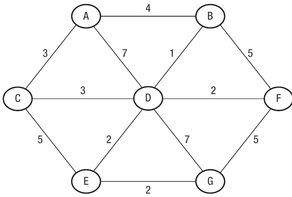
The diagram above shows a more complex network with multiple vertices and edges – exactly the type of problem where trial and error becomes impractical, making Dijkstra's algorithm essential.

Tracing Dijkstra's algorithm step-by-step

Now let's learn how to trace Dijkstra's algorithm by hand – this is a key skill for your exam. We'll use a worked example to understand each step of the process.

The algorithm overview:

The algorithm follows these main steps:

Start from your chosen initial vertex (in our example, we'll use vertex A)
Calculate the weight (cost) for each edge connecting that vertex to other connected vertices
Move to the nearest unvisited vertex and repeat the process, adding weights together to get total distances
When you have multiple route options to the same vertex, always keep the shortest distance
Mark vertices as "visited" once you've processed them, and don't recalculate their distances
Continue until all vertices have been visited, and you've reached your destination

lightbulbExample

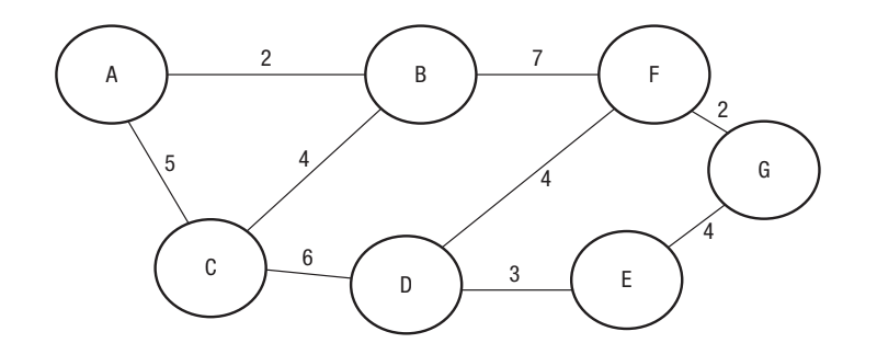
Worked Example: Finding the Shortest Path from A to G

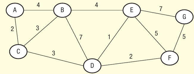
Let's trace the algorithm to find the shortest path between vertex A and vertex G in the following graph:

We'll record our progress in a table. This systematic approach helps you keep track of the shortest known distance to each vertex as the algorithm progresses.

Table

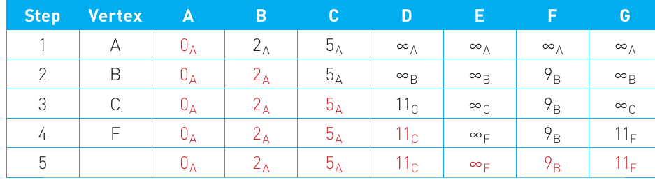
Step 1 – Starting from vertex A:

Place vertex A in the first column. Now calculate the distance from A to every other vertex it connects to:

A to A = 0 (you're already there!)
A to B = 2
A to C = 5
All other vertices cannot be reached directly from A, so we mark them with infinity (∞)

Notice that each distance has a subscript letter A. This subscript tells us which vertex we travelled from to reach that distance. This will become important later when we need to reconstruct the actual path.

Step 2 – Moving to vertex B:

Look at the previous row and identify which unvisited vertex has the smallest distance from A. It's vertex B with a distance of 2. Mark B in the vertex column.

Now we need to update the distances for all vertices that B connects to:

Distance to A remains $0_A$ (already processed)
Distance to B remains $2_A$ (we've arrived here)
Distance to C: We can go A → B → C, which would be $2 + 4 = 6$ . However, we already know that going directly from A to C is 5, which is shorter. So we keep $5_A$
Distance to F: A → B → F would be $2 + 7 = 9_B$
All other vertices remain at infinity

The key principle here is: always keep the shortest distance you've found so far.

Step 3 – Moving to vertex C:

The next smallest unvisited distance is 5 (to vertex C). Notice that in the table, vertices we've already dealt with (A and B) are shown in red to indicate they're "locked" – we won't change their values again.

Distance to A: $0_A$ (locked)
Distance to B: $2_A$ (locked)
Distance to C: $5_A$ (we've arrived)
Distance to D: A → C → D would be $5 + 6 = 11_C$
All other distances stay the same for now

Step 4 – Moving to vertex F:

The next smallest unvisited distance is 9 (to vertex F). Complete the table entries:

Distance to A: $0_A$ (locked)
Distance to B: $2_A$ (locked)
Distance to C: $5_A$ (locked)
Distance to D: $11_C$ (no change)
Distance to E: $\infty \rightarrow \infty_F$ (F doesn't connect to E)
Distance to F: $9_B$ (we've arrived)
Distance to G: A → B → F → G would be $9 + 2 = 11_F$

Note that we skipped considering vertices D and E in this step. The algorithm recognises that since we're looking for the shortest path, and the distance to D (11) is already greater than the shortest distance to G found so far, D cannot be on the shortest path to G.

Step 5 – Final step:

There are no more edges to compare, so we list the final values. Looking at the last row of the table:

The shortest distance from A to G is 11
The subscript letters tell us the path: A → B → F → G (by reading the subscripts: $11_F$ means we came from F, $9_B$ means we got to F from B, and $2_A$ means we got to B from A)

You can verify this is correct by checking alternative routes:

A → C → D → E → G would be $5 + 6 + 3 + 4 = 18$
A → C → B → F → G would be $5 + 4 + 7 + 2 = 18$

Both alternatives are longer than our answer of 11, confirming we found the shortest path.

Implementing Dijkstra's algorithm with arrays

For your exam and coursework, you need to understand how Dijkstra's algorithm can be implemented in a programming language. The most efficient way to represent a weighted graph in code is using a two-dimensional array (also called an adjacency matrix).

Using a two-dimensional array:

Consider a graph with seven vertices (A through G). We can represent all the connections and their weights in a 7×7 array:

infoNote

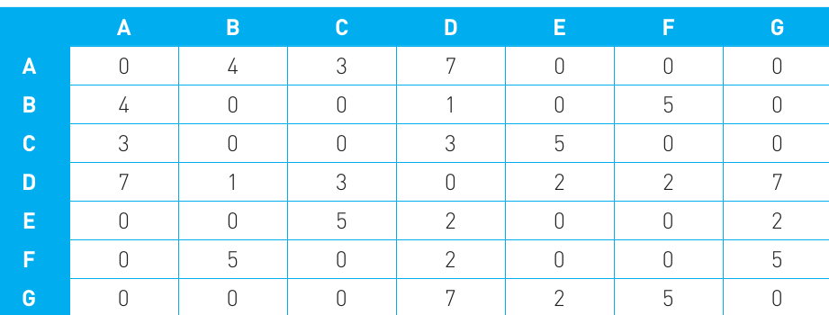
Understanding the Adjacency Matrix:

In this array representation:

Rows represent the "from" vertex
Columns represent the "to" vertex
The number at each intersection represents the weight of the edge between those vertices
A value of 0 appears where a vertex connects to itself
The array is symmetric for an undirected graph (the value at position [A,B] equals the value at position [B,A])

This array represents the following graph:

Key data structures needed:

To implement Dijkstra's algorithm, you need several arrays and variables to track information:

MinDist array: Stores the shortest known distance from the start vertex to each vertex
NodeFixed array: A Boolean array marking which vertices have been fully processed
Route array: Stores the path taken to reach each vertex
RouteMatrix: The two-dimensional array containing the graph's edge weights
NodeCount: The total number of vertices in the graph

Implementation overview:

The implementation follows this general approach:

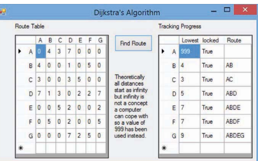
Initialise: Set up your arrays. Use a large number (like 999) to represent infinity, as computers can't handle the mathematical concept of infinity directly.
Load the graph data: Read the edge weights from a file or data source into your two-dimensional array.
Start the recursive process: Begin from your starting vertex (distance = 0).
Process each vertex:
- Mark the current vertex as fixed (processed)
- For each unfixed vertex connected to the current vertex, calculate: potential new distance = current vertex's distance + edge weight
- If this new distance is shorter than the previously known distance, update it
- Record which vertex the path came from
Find the next vertex: Among all unfixed vertices, find the one with the smallest distance and process it next.
Repeat: Continue until all vertices are fixed or you've reached your destination.
Extract the path: Use the route information to reconstruct the shortest path.

The code maintains a tracking table showing the progress of the algorithm, similar to the manual tracing tables we used earlier. This helps verify the algorithm is working correctly and makes it easier to debug.

chatImportant

Important Implementation Notes:

The algorithm uses recursion to visit each node systematically
Using 999 instead of infinity is a practical compromise – just ensure this value is larger than any possible actual path distance in your graph
The "locked" (or "fixed") status prevents the algorithm from recalculating vertices unnecessarily, making it more efficient
Keeping track of the route (which vertex you came from) is essential for reconstructing the final path

Exam tips and common pitfalls

Exam tips:

Show your working: Always use a table when tracing Dijkstra's algorithm by hand. Examiners want to see your systematic approach, not just the final answer.
Use subscripts: Remember to include subscript letters showing which vertex you travelled from. This demonstrates you understand how the algorithm tracks the path.
Mark processed vertices: Cross out or highlight vertices once they're locked/fixed. This helps you avoid recalculating them.
Check edge weights carefully: A simple misreading of an edge weight can throw off your entire answer. Double-check the graph.
Start with the smallest: Always move to the unvisited vertex with the smallest known distance from the start.
Remember: positive weights only: Dijkstra's algorithm doesn't work correctly with negative edge weights. If asked about limitations, mention this.

chatImportant

Common Pitfalls to Avoid:

Forgetting to add cumulative distances: When calculating distances via intermediate vertices, you must add the distance to the intermediate vertex plus the edge weight to the next vertex.
Updating already-fixed vertices: Once a vertex is marked as fixed/locked, its distance value should not change.
Not keeping the shortest distance: If you find multiple routes to the same vertex, always keep the one with the smallest total distance.
Confusing directed and undirected graphs: Make sure you understand whether edges can be travelled in both directions or just one.
Mixing up infinity notation: Be consistent with how you represent infinity (∞ or a large number like 999).

Understanding algorithm limitations

While Dijkstra's algorithm is powerful, it's important to understand what it cannot do:

infoNote

Algorithm Limitations:

Not suitable for the travelling salesman problem: Dijkstra's algorithm finds the shortest path between two points but doesn't solve the travelling salesman problem, which asks: "What's the shortest route that visits every vertex exactly once and returns to the start?" This is a different type of problem requiring different algorithms.

Requires positive weights: The algorithm assumes all edge weights are positive. If your graph has negative weights, you need a different algorithm (like Bellman-Ford).

Single metric optimisation: The algorithm optimises for one metric at a time (distance, time, cost, etc.). If you need to consider multiple factors simultaneously, you'd need a more complex approach.

bookmarkSummary

Key Points to Remember:

Dijkstra's algorithm finds the shortest path from a single starting vertex to all other vertices in a weighted graph, using a systematic approach that guarantees the optimal solution.
The algorithm works iteratively: starting from the source vertex, it always moves to the nearest unvisited vertex, calculating and updating distances as it goes. Once a vertex is marked as "fixed" or "locked", its distance never changes.
Use a table for manual tracing: Include columns for each vertex, show the step number, mark which vertex you're currently processing, and use subscripts to track which vertex each path came from. Mark completed vertices clearly.
Real-world applications are everywhere: from sat-nav systems calculating driving routes, to internet routers directing data packets, to logistics companies planning delivery routes – Dijkstra's algorithm solves practical problems every day.
Implementation uses 2D arrays: the most efficient way to represent a weighted graph in code is using a two-dimensional array (adjacency matrix), along with supporting arrays to track distances, visited status, and routes. Remember to use a large number like 999 to represent infinity in your code.

Dijkstra’s Shortest Path Algorithm (AQA A-Level Computer Science): Revision Notes