Graph and Tree Traversal Revision Notes for AQA A-Level Computer Science

Graph and Tree Traversal

Introduction to graph and tree traversal

When working with graphs and trees in computer science, you need to be able to move through them systematically to access or process all the data they contain. This process is called traversal, which means visiting every node in the structure in a specific order. Just like reading a book page by page, traversing means moving across a data structure, but unlike reading, there are different ways to do it depending on what you need to achieve.

Understanding traversal is essential because these algorithms form the foundation of many practical applications, from search engines exploring web pages to file systems organizing directories. In this note, we'll explore how to implement graphs, then learn two main methods for traversing graphs (depth first and breadth first), followed by three methods for traversing binary trees (pre-order, in-order, and post-order). Finally, we'll look at recursion, a powerful technique that makes many traversal algorithms elegant and efficient.

infoNote

Traversal algorithms are fundamental to computer science and appear in countless real-world applications. Mastering these concepts will help you understand how search engines work, how file systems are organized, and how many optimization problems are solved.

Implementing a graph

Before you can traverse a graph, you need to understand how graphs are stored in computer memory. A graph is a data structure consisting of nodes (also called vertices) connected by edges. Think of it like a network of cities (nodes) connected by roads (edges).

There are two main ways to represent a graph in code:

Adjacency lists

An adjacency list shows each node alongside all the nodes that are directly connected to it. This is like having a directory where each person lists all their friends.

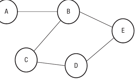
For the graph shown above, we can create an adjacency list that maps each node to its neighbours:

infoNote

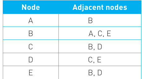
This representation is memory-efficient because you only store the connections that actually exist. If a node has few connections, you don't waste space storing information about non-existent edges. This makes adjacency lists ideal for sparse graphs (graphs with relatively few connections).

Adjacency matrices

An alternative method is to use a two-dimensional array called an adjacency matrix. This is a grid where both rows and columns represent nodes, and each cell contains either a 1 (meaning there's an edge between those two nodes) or a 0 (meaning there's no edge).

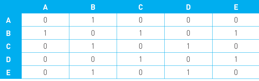
In this matrix, a value of 1 indicates that an edge exists between the two vertices, while 0 means there's no direct connection. This approach works well for representing any unweighted, undirected graph, where all edges have equal importance and connections work in both directions.

chatImportant

Choosing the Right Representation:

The choice between adjacency lists and matrices depends on your needs:

Use adjacency lists for sparse graphs (few connections) - better memory efficiency
Use adjacency matrices for dense graphs (many connections) or when you need fast edge lookups - checking if a specific edge exists is O(1)

Traversing a graph

Once you've implemented a graph, you'll often need to explore it to find specific information or process all the nodes. There are two fundamental approaches to graph traversal: depth first and breadth first.

Depth first traversal

Depth first is a method that explores as far as possible along each path before backtracking. Imagine you're exploring a maze - you'd follow one corridor all the way to the end before turning back and trying a different route.

Here's how depth first traversal works:

Start at a chosen node and mark it as visited
Choose an adjacent unvisited node and recursively explore from there
When you reach a node with no unvisited neighbours, backtrack to the previous node
Continue until all reachable nodes have been visited

lightbulbExample

Worked Example: Depth First Traversal

Consider a simple graph with nodes A, B, C, D connected as: A→B, A→C, B→D

Starting from node A:

Visit A (mark as visited)
Move to B (recursive call)
- Visit B (mark as visited)
- Move to D (recursive call)
  - Visit D (mark as visited)
  - No unvisited neighbours, return to B
- No more unvisited neighbours from B, return to A
Move to C (recursive call)
- Visit C (mark as visited)
- No unvisited neighbours, return to A
All nodes visited

Result: A → B → D → C

This approach uses recursion, where the algorithm calls itself repeatedly. Each time you move to a new node, you make another recursive call. The beauty of this method is that the computer automatically handles the backtracking by using the call stack to remember where you've been.

Breadth first traversal

Breadth first takes a different approach - it explores all nodes at the current "distance" from the starting point before moving further away. Think of it like ripples spreading out in a pond, exploring each ring completely before moving to the next ring.

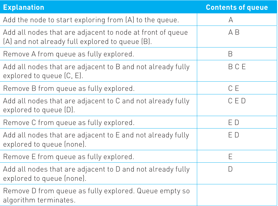
The algorithm uses a queue (a first-in, first-out data structure) to keep track of which nodes to visit next. Here's the process:

Add your starting node to the queue and mark it as visited
Remove the first node from the queue (this becomes your current node)
Add all unvisited adjacent nodes to the queue and mark them as visited
Repeat steps 2-3 until the queue is empty

infoNote

Breadth first traversal guarantees that you'll find the shortest path between two nodes in an unweighted graph, making it particularly useful for pathfinding algorithms and determining the minimum number of steps needed to reach a goal.

chatImportant

Key Difference Between Depth First and Breadth First:

Depth first goes deep into one path before exploring others (uses recursion and the call stack)
Breadth first explores all nearby options before venturing further away (uses a queue data structure)

Choose depth first when you want to explore all possible paths or when memory is a concern. Choose breadth first when you need to find the shortest path or when solutions are likely to be found close to the starting point.

Traversing a binary tree

A binary tree is a special type of tree structure where each node can have at most two children - a left child and a right child. Tree traversal extracts all the data from the tree in some particular order. Unlike graphs, trees have a hierarchical structure with a clear starting point (the root) and no cycles.

There are three main methods for traversing binary trees, each producing a different ordering of the nodes:

Pre-order traversal

In pre-order traversal, you visit each node according to this pattern:

Visit the current node (process or output its data)
Traverse the left subtree
Traverse the right subtree

infoNote

This is useful when you want to process parent nodes before their children, such as when copying a tree structure or evaluating prefix notation expressions (where operators come before their operands).

In-order traversal

In in-order traversal follows this pattern:

Traverse the left subtree
Visit the current node
Traverse the right subtree

chatImportant

In-Order Traversal and Binary Search Trees:

This method is particularly important because when applied to a binary search tree, it produces nodes in sorted order. This makes in-order traversal equivalent to performing a binary search on the tree, which is an efficient way to find data by repeatedly dividing the search space in half.

No matter how you arrange the data in a binary search tree, an in-order traversal will always produce a sorted list.

Post-order traversal

Post-order traversal uses this pattern:

Traverse the left subtree
Traverse the right subtree
Visit the current node

This approach is useful when you need to process children before their parents, such as when deleting nodes from a tree or evaluating postfix notation expressions (Reverse Polish Notation). It can also be used to empty a tree by processing all descendant nodes before removing parent nodes.

infoNote

Memory Aid for Tree Traversal:

The name tells you when to visit the node:

"Pre" means before traversing subtrees
"In" means in between the left and right subtrees
"Post" means after traversing both subtrees

An interesting property of in-order traversal is that no matter how you arrange the data in a binary search tree, an in-order traversal will always produce a sorted list. However, pre-order and post-order will produce different sequences if the data is rearranged in the tree.

Recursion

Recursion is a programming technique where a function calls itself to solve a problem. While this might sound confusing at first, it's actually an elegant way to solve problems that have a repetitive or self-similar structure, like traversing trees.

The tree traversal algorithms we've discussed all use recursion. When the traverse function is called, it processes the current node and then calls itself to process child nodes. Each function call operates on a smaller part of the tree until eventually there are no more nodes to visit.

chatImportant

Two Essential Components of Recursion:

For recursion to work properly, you need:

Base case (terminating condition): This defines when the recursive function should stop calling itself. For tree traversal, the base case is when there are no more child nodes to visit. Without a base case, the function would call itself forever, causing a stack overflow error.
General case: This defines how the function calls itself with modified parameters. In tree traversal, the general case involves calling the traverse function on the left or right child nodes.

Here's how recursion works for in-order tree traversal:

lightbulbExample

Worked Example: Recursive In-Order Traversal

Define Procedure Traverse
    If there is a node to the left Then
        Go Left
        Traverse
    End If
    Visit
    If there is a node to the Right Then
        Go Right
        Traverse
    End If
End Procedure

How it works:

When you call this procedure on a tree:

It checks if there's a left child
If there is, it moves left and calls Traverse again (recursive call)
The computer stores the current position on the call stack and jumps to the new position
Eventually, when you reach a node with no left child, the base case is triggered (the If statement is false)
You process that node (Visit)
Then the function checks for a right child and recurses again if one exists
The stack automatically handles all the bookkeeping of where you've been and where you need to return to

Each recursive call adds a layer to the stack, and each return removes a layer.

This is why recursive algorithms are often much shorter and clearer than their iterative equivalents, though they do use more memory because of the stack.

infoNote

Understanding recursion is crucial for computer science because many algorithms, from tree traversals to sorting methods like quicksort and mergesort, rely on this technique. The key insight is that complex problems can often be broken down into simpler instances of the same problem, which is exactly what recursion enables you to do.

Remember!

bookmarkSummary

Key Points to Remember:

Graphs can be represented using adjacency lists or adjacency matrices - lists show each node with its neighbours, while matrices use a 2D array of 0s and 1s to show connections
Depth first traversal explores as far as possible along each branch before backtracking - it uses recursion and is good for exploring all possible paths
Breadth first traversal explores nodes level by level, visiting all neighbours before moving further away - it uses a queue and finds the shortest path in unweighted graphs
Binary trees have three traversal methods: pre-order (visit-left-right), in-order (left-visit-right), and post-order (left-right-visit) - in-order produces sorted output for binary search trees
Recursion is when a function calls itself, requiring a base case to stop and general cases to continue - it's used extensively in tree traversal algorithms and makes code more elegant and easier to understand

Graph and Tree Traversal (AQA A-Level Computer Science): Revision Notes