Graphs and Trees (AQA A-Level Computer Science): Revision Notes
Graphs and Trees
Introduction to graphs
A graph is a special mathematical structure used to model how different objects or items relate to one another. In graph theory, we study the underlying mathematical principles that help us understand and work with these structures. Graphs are incredibly useful in computing because they allow us to represent complex real-life situations in a way that computers can process and analyse.
Think of a graph as being made up of two main components:
- Vertices (also called nodes): These are the objects or points in your graph. For example, they could represent towns, people, or websites.
- Edges (also called arcs): These are the connections or relationships between the vertices. They show how one vertex relates to another.
The terms vertices and nodes are interchangeable, as are edges and arcs. Different textbooks and contexts may use different terminology, but they refer to the same concepts.
Let's start with a simple example. Imagine we want to show the connection between two towns. We can represent each town as a vertex (a circle), and the connection between them as an edge (a line):
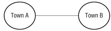
This basic graph shows that Town A and Town B are connected in some way, perhaps by a train line or road.
Weighted graphs
Often, we need more information than just "these two things are connected". We might want to know the distance, travel time, or cost associated with that connection. This is where weighted graphs become useful.
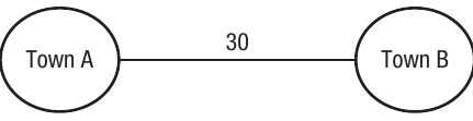
A weighted graph has numerical values attached to each edge. These values (called weights) provide additional information about the relationship between vertices. For example, if we add the travel time of 30 minutes between our two towns, the graph becomes:
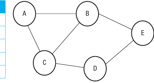
Let's extend this to a more realistic scenario with multiple towns. The following graph shows a transport network with five towns and the journey times between them:
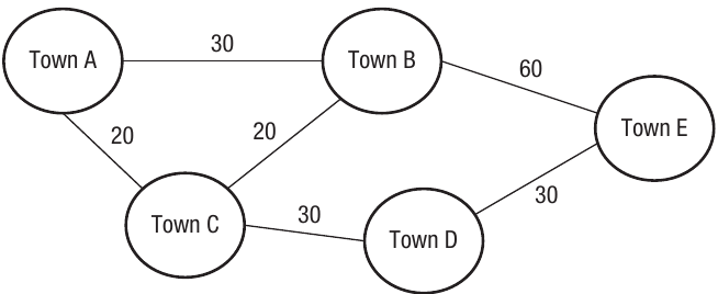
Notice that not all towns are directly connected to each other. For instance, there's no direct connection shown between Town A and Town E. If you wanted to travel from Town A to Town E, you would need to go via other towns.
Worked Example: Finding the Quickest Route
To travel from Town A to Town E, we have two possible routes:
Route 1: Via Towns C and D
- Town A → Town C: 20 minutes
- Town C → Town D: 30 minutes
- Town D → Town E: 30 minutes
- Total time: 20 + 30 + 30 = 80 minutes
Route 2: Via Town B
- Town A → Town B: 30 minutes
- Town B → Town E: 60 minutes
- Total time: 30 + 60 = 90 minutes
Therefore, Route 1 via Towns C and D is the quickest route at 80 minutes.
Directed vs undirected graphs
Graphs can show relationships that work in different ways:
Undirected graphs
An undirected graph represents relationships that work in both directions equally. In the towns example above, the trains go in both directions—you can travel from Town A to Town B and also from Town B to Town A. The relationship is two-way, so the edges have no arrows.
Directed graphs
A directed graph (also called a digraph) represents one-way relationships. The edges have arrows showing the direction of the relationship. This is useful for modeling situations where the relationship only works one way.
For example, consider a family tree showing parent-child relationships:
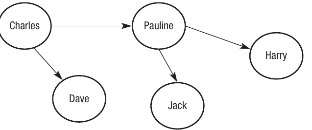
The arrows indicate that Charles is the parent of Dave and Pauline, and Pauline is the parent of Harry and Jack. The relationship only goes in one direction—a parent "points to" their children, but not the other way around.
In directed graphs, the direction of the arrow is crucial. An edge from A to B does not imply an edge from B to A. This makes directed graphs perfect for representing relationships like "is the parent of", "follows on social media", or "links to" on the web.
Uses of graphs
Graphs have numerous practical applications in computing and the real world:
Human networks
Social networks like LinkedIn are perfect examples of graph structures. Each person is a vertex, and each connection between people is an edge. When you add someone as a contact, you create an edge between your vertex and theirs. The network grows as people connect with others who connect with more people, creating a vast interconnected graph.
Transport networks
All transport systems work on the principle of graphs. Departure points and arrival points are vertices, whilst routes between them are edges. Graph theory helps transport planners to:
- Calculate the quickest routes between locations
- Plan timetables efficiently
- Schedule staff effectively
- Optimise network coverage
The internet and web
The Internet itself can be mapped as a massive graph structure. Each connected device is a vertex, with physical connections forming the edges. Similarly, the World Wide Web is a graph where each website is a node and each hyperlink to another site forms an edge.
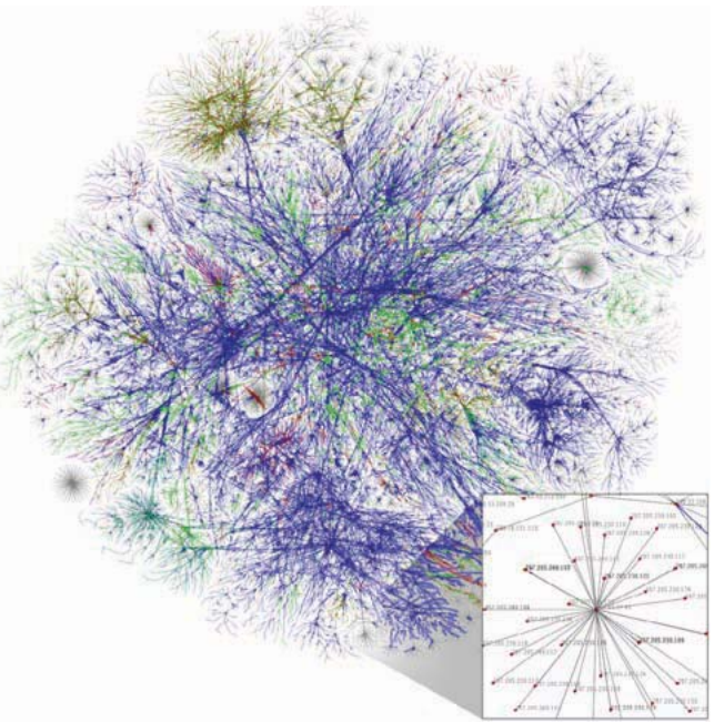
Notice how the Internet map looks more like a complex web radiating from central points. The concentrations of color show where Internet Service Providers (ISPs) route large amounts of data through their servers.
Computer science and latency
Latency refers to the time delay that occurs when transmitting data between devices. Graph theory helps calculate the quickest path to send data around a microprocessor, where each vertex represents a processor component and edges represent the buses that carry the data.
Medical research
Understanding how diseases spread is crucial for prevention. Each case of a disease (or each location where outbreaks occur) can be a vertex, with edges showing the connections between cases. Weighted graphs help analyze how far and how quickly diseases spread between different locations.
Weighted graphs are particularly valuable in epidemiology. The weights can represent factors like distance between cases, time between transmissions, or the strength of contact between infected individuals, helping researchers model and predict disease spread patterns.
Project management
Large-scale projects (engineering, construction, or IT) can be modeled using graphs. Each task needed to complete the project is a vertex, and the edges show the relationships and dependencies between tasks. This helps project managers understand which tasks must be completed before others can begin.
Game theory
In strategic games and conflict situations, graphs help predict possible actions and outcomes. The vertices represent actions that might be taken, and the edges represent the possible outcomes or consequences of those actions.
Dijkstra's algorithm
Graph theory is essential for Dijkstra's algorithm, which calculates the shortest path between nodes. This has been used for applications such as calculating shortest distances between cities and finding shortest routes between vertices in computer networks. (This is covered in more detail in Chapter 13.)
Representing graphs with adjacency lists
Whilst drawing graphs is helpful for understanding them visually, computers need a structured way to store and process this information. The first method we'll look at is the adjacency list.
The term adjacent means "next to", so an adjacency list stores each vertex along with information about which vertices are next to it (connected to it by an edge). The format of the list depends on whether the graph is directed or undirected, and whether it's weighted.
Adjacency list for an undirected graph
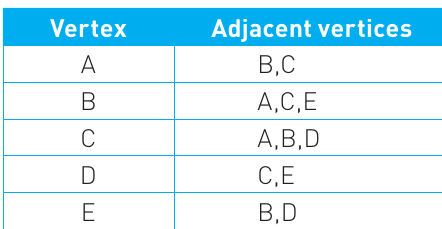
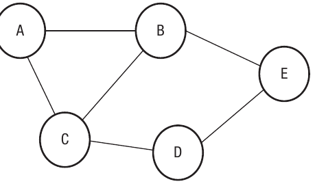
The table lists each vertex in the left column and shows all the vertices connected to it in the right column. Since this is an undirected graph, all connections are two-way. For example, vertex A is connected to B and C, so both B and C appear in A's row. Similarly, since A connects to B, you'll also find A listed in B's row.
In adjacency lists for undirected graphs, every connection appears twice—once in each vertex's row. If A is connected to B, then B appears in A's list AND A appears in B's list. This redundancy is necessary to represent the two-way nature of undirected edges.
Adjacency list for a directed graph
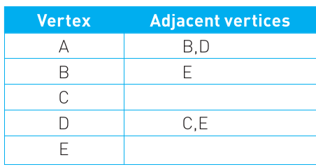
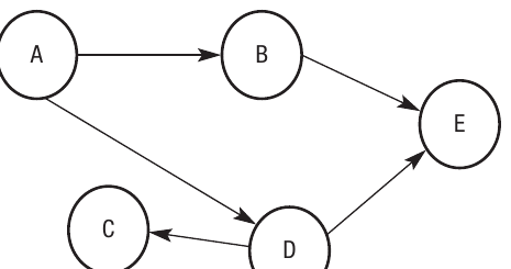
For directed graphs, the list only shows the one-way relationships. The arrows in the diagram indicate direction. For example, vertex A has arrows pointing to B and D, so B and D are listed as adjacent to A. However, D connects to C and E, but C isn't connected to D in return—C has no outgoing edges, so its row is empty.
Adjacency list for a weighted graph
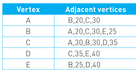
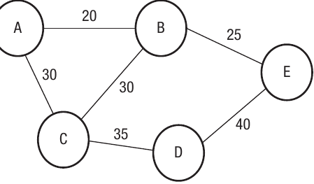
When graphs have weights, the adjacency list includes both the connected vertex and the weight value. For instance, vertex A is connected to B with a weight of 20, and to C with a weight of 30, so the entry for A shows "B,20,C,30". This format allows the computer to store both which vertices are connected and what the connection weight is.
Representing graphs with adjacency matrices
The second method for storing graph data is to use an adjacency matrix. This is a two-dimensional array (a grid or table) that shows whether edges exist between each pair of vertices. The rows and columns both represent vertices, and the values in the cells show whether connections exist.
Adjacency matrix for an undirected graph
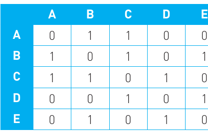
The matrix works by placing a 1 in each cell where there's an edge between two vertices, and a 0 where there isn't. For example, vertex A is connected to vertex B, so there's a 1 where row A and column B intersect. Similarly, there's a 1 where row B and column A intersect (because it's undirected). Vertex A is not connected to vertex D, so there are 0s at the A-D and D-A positions.
Adjacency matrices for undirected graphs are always symmetrical along the diagonal. This means if there's a 1 at position (A, B), there will also be a 1 at position (B, A). The diagonal itself (A-A, B-B, etc.) typically contains 0s since vertices don't connect to themselves.
Adjacency matrix for a directed graph
For directed graphs, you read the matrix row by row. A 1 indicates a one-way relationship from the row vertex to the column vertex, and a 0 indicates no relationship. For example, vertex A has arrows pointing to B and D, so row A has 1s in the B and D columns. However, B doesn't point back to A, so row B has a 0 in the A column.
Adjacency matrix for a weighted graph
For weighted graphs, instead of using 1s and 0s, we place the actual weight value in each cell. Where there's no connection, the infinity symbol () is used instead of 0. This makes sense because infinity represents an impossibly large distance or cost—essentially meaning "no connection exists". For example, A connects to B with a weight of 20, so the cell at row A, column B contains 20.
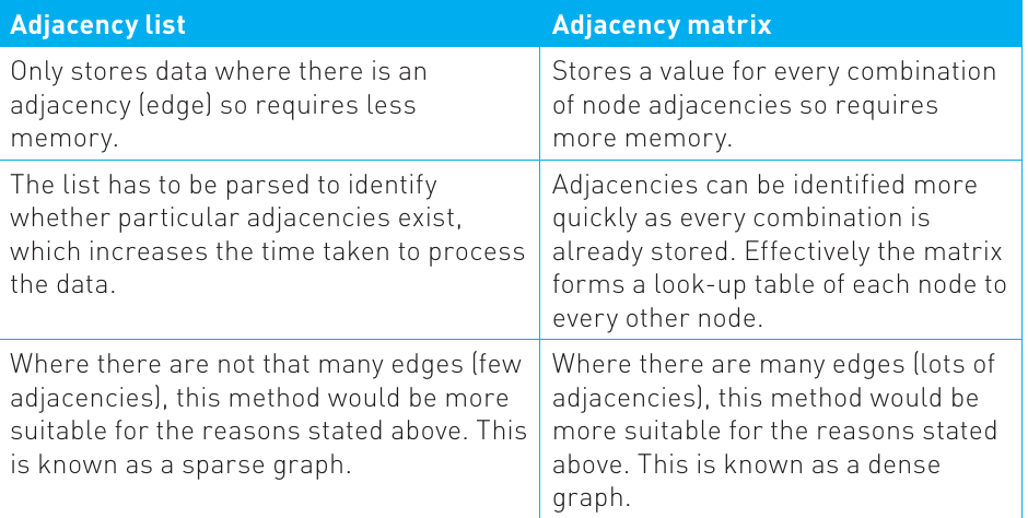
Adjacency list vs adjacency matrix
Both methods have their advantages and disadvantages, and choosing between them depends on your specific needs. The decision usually comes down to two factors: speed and memory.
Speed refers to how quickly your program can access the data structure and produce results. Memory refers to the amount of storage space the implementation requires.
Consider that graph structures often deal with very large datasets. In the simple examples we've looked at, five vertices produce 25 cells in a matrix but might only need storage for 6-10 edges in an adjacency list.
Worked Example: Comparing Storage Requirements
5 vertices:
- Matrix: cells
100 vertices:
- Matrix: cells
1,000 vertices:
- Matrix: cells
If each cell requires just one byte of storage, that's already a 1 MB file. With thousands or millions of vertices, file sizes can become enormous.
Key considerations when choosing between adjacency lists and matrices:
-
Adjacency lists use less memory because they only store data where edges actually exist. This is particularly efficient for sparse graphs (graphs with relatively few connections).
-
Adjacency matrices provide faster lookups because you can identify whether two vertices are adjacent instantly by checking a single cell. With lists, you need to parse through the list to find the information.
-
Lists are better for sparse graphs (few edges relative to vertices), whilst matrices are better for dense graphs (many edges).
Trees
A tree is a special type of graph that shares similarities with standard graphs but has some important differences. Like graphs, trees are made up of nodes (vertices) and edges (connections between nodes). They're called "trees" because when visualized, they look like hierarchical structures with branches, similar to a family tree.
The key characteristics that distinguish trees from general graphs are:
- Trees are connected—you can reach any node from any other node
- Trees are undirected
- Trees contain no cycles or loops
What does "no cycles" mean? In a graph, if you can travel from vertex A to vertex B to vertex C and back to vertex A, you've created a cycle. In a tree, this isn't possible. You might go from A to B and from B to C, but you cannot return to A via C. This creates a one-way branching structure.
Here's a simple tree structure:
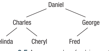
In this family tree, Daniel is at the top with two children: Charles and George. Charles has two children (Belinda and Cheryl), whilst George has one child (Fred). Notice that you cannot create a loop—there's no way to travel from one person back to themselves by following the tree branches.
Tree terminology
Trees have specific terminology to describe different parts of their structure:
- Root node: The starting point of the tree from which all other nodes branch away. In the example above, Daniel is the root.
- Parent node: A node that has other nodes (children) below it in the hierarchy. Charles is a parent to Belinda and Cheryl.
- Child node: A node that has a node above it (a parent). Belinda and Cheryl are children of Charles.
- Leaf node: A node that has no children below it. Belinda, Cheryl, and Fred are all leaf nodes.
Uses of trees
Trees have several important applications in computing:
Storing hierarchical data: Trees naturally represent data that has an inherent hierarchical structure. For example, operating systems use tree structures for their file management systems, where folders contain subfolders and files.
Dynamic structures: Trees make it easy to add and delete nodes as needed, making them flexible for changing datasets.
Searching and sorting: Trees can be searched and sorted efficiently using standard traversal algorithms (covered in Chapter 16).
Processing syntax: Trees are commonly used to process the syntax of statements in natural languages and programming languages, making them essential for compilers and interpreters.
Binary search trees
A binary tree is a specific type of tree where each node can have a maximum of two child nodes attached to it. This "binary" limit (meaning two) creates a structure that's particularly efficient for certain operations.
Binary search trees are commonly used to store data that arrives in random order. The beauty of the structure is that data automatically becomes sorted as it's entered. The tree can then be "traversed" (walked through in a specific order) to search for and extract data efficiently.
How binary trees work
When adding data to a binary tree, the first item becomes the root node. Each subsequent item is added according to a simple rule:
Binary Tree Insertion Rule:
- If the new value is less than the current node's value, branch left
- If the new value is greater than or equal to the current node's value, branch right
- Keep following this rule until you reach an empty branch, then place the new value there
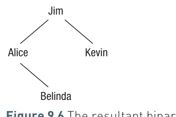
Let's see how this works with an example. Starting with "Jim" as the root, we'll add "Kevin", "Alice", and "Belinda":
Worked Example: Building a Binary Tree
Step 1: Jim becomes the root node (the first item always becomes the root)
Step 2: Adding Kevin
- Kevin > Jim, so branch right
- Right branch is empty, so Kevin is placed as Jim's right child
Step 3: Adding Alice
- Alice < Jim, so branch left
- Left branch is empty, so Alice is placed as Jim's left child
Step 4: Adding Belinda
- Belinda < Jim, so branch left (we move to Alice)
- Belinda > Alice, so branch right from Alice
- Right branch is empty, so Belinda is placed as Alice's right child
Implementing a binary tree with arrays
To implement a binary tree in code, we need three arrays:
- Node array: Stores the actual data values
- Left array: Stores which node is the left child of each node
- Right array: Stores which node is the right child of each node
Here's how the binary tree above would be represented:
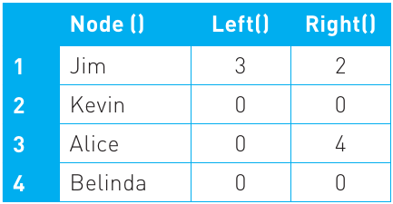
The numbers in the Left and Right columns are index positions pointing to other nodes. A value of 0 indicates an empty branch (no child node exists there). This pointer-based approach allows the tree structure to be represented using simple arrays.
Algorithm for adding to a binary tree
Here's the algorithm for adding new data to a binary tree:
'Find next gap in the Node array
NodeCount ← 1
While Node(NodeCount) is not empty
    NodeCount ← NodeCount + 1
End While

'NodeCount stores the next blank
Node(NodeCount) ← AddItem

'Start at the root node
PresentNode ← 1
While Node(PresentNode) is not empty do
    'Branch Left or Right?
    If AddItem < Node(PresentNode) Then
        'If Left branch is empty then assign NodeCount
        If Left(PresentNode) = 0 Then
            Left(PresentNode) ← NodeCount
        End If
        PresentNode ← Left(PresentNode)
    Else
        'If Right branch is empty then assign NodeCount
        If Right(PresentNode) = 0 Then
            Right(PresentNode) ← NodeCount
        End If
        PresentNode ← Right(PresentNode)
    End If
End While
If we start with Jim as the root and add Kevin, Alice, and Belinda, the arrays would look like this:
And the resulting tree structure would be:
The algorithm efficiently places each new value in the correct position, maintaining the binary search tree property where smaller values are always to the left and larger values are always to the right.
Key Points to Remember:
-
Graphs consist of vertices (nodes) and edges (arcs) that model relationships between objects, making them essential for representing complex real-world situations in computing.
-
Graphs can be directed, undirected, or weighted depending on whether relationships are one-way or two-way, and whether edges carry additional information like distance or cost.
-
Adjacency lists and adjacency matrices are two ways to represent graphs in code—lists use less memory and are better for sparse graphs, whilst matrices provide faster lookups and are better for dense graphs.
-
Trees are special connected graphs with no cycles, structured hierarchically with a root node, parent nodes, child nodes, and leaf nodes—they're perfect for representing hierarchical data like file systems and family trees.
-
Binary trees limit each node to maximum two children, allowing data to be automatically sorted as it's added and enabling efficient searching through tree traversal algorithms.