The Nature of Supply Revision Notes for Edexcel A-Level Economics A

The Nature of Supply

Introduction to supply

Supply focuses on the behaviour of firms rather than consumers. While demand examines what consumers are willing to purchase, supply considers what producers are willing to sell. In any market transaction, there are two sides: buyers and sellers. Understanding supply helps us identify the factors that determine how much output sellers are prepared to bring to the market.

What is supply?

Supply refers to the quantity of a good or service that producers are willing and able to sell at any given price during a specific time period.

infoNote

The phrase "willing and able" is crucial - it's not enough for producers to simply want to sell; they must also have the capacity to produce and deliver the goods or services to the market.

The role of firms

A firm is an organisation that combines various factors of production to create output. Firms can take different forms:

Sole proprietor: A small business where the owner also manages operations, such as a newsagent
Partnership: A business structure where profits and debts are shared between partners, such as a dental practice
Joint stock company: Larger firms owned by shareholders, which can be either private or public. Public joint stock companies have their shares traded on the stock exchange, whereas private companies do not

The profit maximisation assumption

When analysing how firms make supply decisions, economists typically assume that firms aim to maximise their profits. Profits are calculated as the difference between a firm's total revenue and its total costs. This assumption helps us understand why firms behave in certain ways when prices change or when other market conditions shift.

The supply curve

Just as the demand curve shows the relationship between price and quantity demanded, the supply curve illustrates the relationship between price and quantity supplied by firms.

Understanding the supply curve

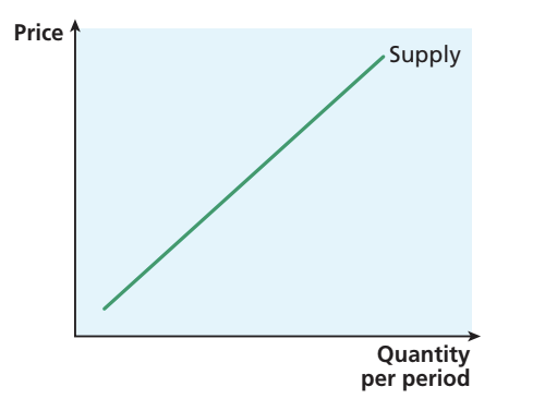
The supply curve shows how much of a product firms in a market are willing and able to supply at different price levels during a given time period. This relationship can be examined for:

An individual firm: showing how much one firm will supply at various prices
The market: showing the total amount all firms in the market will supply at various prices

infoNote

In a competitive market, individual firms cannot influence the price of goods or services they sell because of competition from other firms. Firms must accept the market price and decide how much to supply based on that price.

The positive relationship between price and quantity supplied

Firms operating in competitive markets typically supply more goods at higher prices than at lower prices (ceteris paribus). This creates a positive relationship between price and quantity supplied. The supply curve slopes upward from left to right, reflecting this relationship.

Why does the supply curve slope upward?

When prices are high, firms can earn greater profits by selling their goods. This makes it more attractive for firms to supply more output. Conversely, at lower prices, profits decrease, making firms less willing to supply large quantities. This explains the upward-sloping nature of the supply curve.

Reading supply curves

When interpreting a supply curve, you need to understand how to read the relationship between price and quantity:

If you select a price on the vertical axis, the quantity that firms are willing to supply can be read from the supply curve
At relatively low prices, firms supply smaller quantities
At higher price levels, firms supply larger quantities
The shape of the supply curve shows the extent to which firms respond to different prices

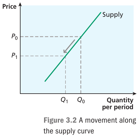
Movement along the supply curve

A change in the price of a good causes firms to adjust their supply decisions, resulting in a movement along the supply curve.

How price changes affect supply

lightbulbExample

Worked Example: Price Changes and Supply Movements

Consider a situation where the price initially sits at $P_0$ , with firms supplying quantity $Q_0$ .

Scenario 1: Price Decrease

If the price falls to $P_1$ , firms find it less profitable to supply the good
They reduce their output, causing a contraction of supply
Quantity supplied falls to $Q_1$
The movement occurs along the existing supply curve

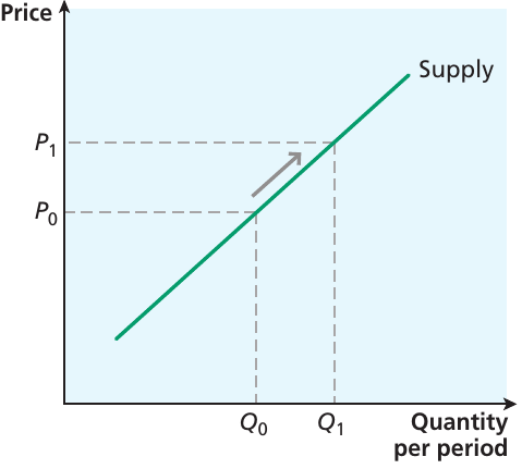
Scenario 2: Price Increase

If the price increases, firms will supply more
This causes an extension of supply
Movement occurs up along the supply curve to a higher quantity

Ceteris paribus condition

The supply curve focuses specifically on the relationship between price and quantity supplied, holding other factors constant. There are various other influences on supply beyond price. When these other factors change, they cause the entire supply curve to shift position rather than creating a movement along it.

What influences supply?

While the supply curve shows how quantity supplied responds to price changes, several other factors determine the position of the supply curve and firms' willingness to supply at any given price:

Production costs
The technology of production
Taxes and subsidies
The price of related goods
Firms' expectations about future prices
The number of firms operating in the market

chatImportant

Make sure you're familiar with all these factors that can influence supply, as they're essential for understanding why supply curves shift. Each factor affects the position of the entire supply curve rather than causing a movement along it.

Costs and technology

Production costs

Production costs represent a major influence on supply decisions. Firms aiming to maximise profits must consider the costs they face when producing output. To create products, firms need to use inputs from the factors of production - labour, capital, land, and so on.

lightbulbExample

Worked Example: Impact of Rising Production Costs

Initial situation:

Firms supply 100 units at £10 per unit

After cost increase:

Production costs increase by £6 per unit
Firms now supply only 50 units at the same price of £10

Result:

The supply curve shifts leftward (from $S_0$ to $S_1$ )
Higher costs make it less profitable to produce
The vertical distance between $S_0$ and $S_1$ represents the £6 cost increase per unit

Technology improvements

New technology can have the opposite effect. If firms introduce more cost-effective production methods, they can produce more output at any given price. This shifts the supply curve to the right.

lightbulbExample

Worked Example: Impact of Technological Improvements

Initial situation:

Firms supply 50 units at £10 per unit

After technology improvement:

Improved technology reduces costs by £6 per unit
Firms can now supply 100 units at the same price of £10

Result:

The supply curve shifts rightward (from $S_0$ to $S_1$ )
Lower costs enable increased production at each price level

Taxes and subsidies

Government policies involving taxes and subsidies also affect supply decisions.

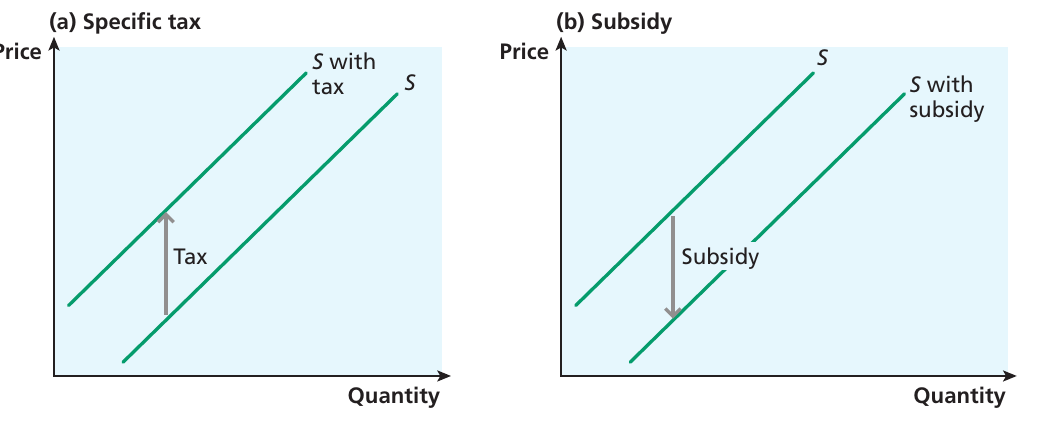
Specific taxes

When the government imposes a sales tax such as VAT, the price consumers pay is higher than the revenue firms receive, as the tax must be paid to the government. This means firms are prepared to supply less output at any given market price (ceteris paribus).

A specific tax is a fixed amount of tax per unit. Such taxes shift the supply curve to the left, as firms supply less at each market price. The vertical distance between the original supply curve and the new "S with tax" curve represents the tax amount per unit.

Subsidies

If the government pays firms a subsidy to produce a particular good, this reduces firms' costs and encourages them to supply more output at any given price. The supply curve shifts to the right. The vertical distance between the curves shows the subsidy amount per unit.

infoNote

The effect of indirect taxes will be discussed in more detail in later chapters after developing the full demand and supply model. Understanding how taxes and subsidies shift the supply curve is crucial for analyzing government intervention in markets.

Prices of other goods

Firms may face situations where they can choose between producing different products, meaning there are alternative uses for their factors of production.

Substitutes in production

If the price of one good increases, it becomes more profitable, potentially encouraging a firm to switch production away from other goods. This may occur even when switching costs are high, provided the price increase is sufficiently large.

lightbulbExample

Example: Substitutes in Production

A change in relative prices of potatoes and organic swedes might encourage a farmer to stop planting potatoes and grow organic swedes instead. If organic swede prices rise significantly, the farmer may reallocate land, labour, and other resources toward the more profitable crop.

Joint supply

In some cases, firms produce multiple goods jointly as by-products of the same production process. For example, a sheep farmer produces both wool and meat from the sheep. An increase in the price of one good may lead the firm to produce more of both goods. This concept of joint supply is similar to complementary goods from the demand side, where consumers regard two goods as complements.

Expected prices

Production takes time, so firms often make supply decisions based on expected future prices rather than current prices alone.

If firms produce goods that can be stored, they may decide to build up stocks in anticipation of higher future prices, potentially holding back some current production. In some economic activities, expectations about future prices are crucial for informing supply decisions because of the length of time needed to increase output.

lightbulbExample

Example: Time Lags in Production

Building firm:

Observes that house prices are increasing in a certain area
Cannot supply new houses immediately because construction takes time
Must base decisions on expected future prices rather than current prices

Wine producer:

Must make supply decisions based on expected future prices
The production process from grape harvest to finished wine is lengthy
Storage costs and aging requirements affect supply decisions

The number of firms in the market

The market supply curve represents the sum of individual firms' supply curves. Therefore:

If more firms enter the market, the market supply curve shifts to the right
If firms exit the market, the market supply curve shifts to the left

This makes intuitive sense: more producers in a market means more total output supplied at any given price, while fewer producers means less total output supplied.

Market power

In some markets, firms may possess market power that enables them to influence the supply of a commodity.

Cartel: An agreement between firms in a market on price and output with the intention of maximising their joint profits.

lightbulbExample

Example: OPEC Oil Cartel

In the oil industry, oil-exporting nations work together as a cartel to influence the quantity supplied. One motivation for this is to influence price and thereby increase the profits of cartel members. By coordinating production levels, cartel members can restrict supply and drive up prices.

infoNote

The operation of cartels is discussed more comprehensively in later chapters on market structures. Cartels represent a significant departure from the competitive market model.

Movements along and shifts of the supply curve: a reminder

It's essential to distinguish between movements along the supply curve and shifts of the supply curve.

Movements along the supply curve

A change in the market price induces a movement along the supply curve (an extension or contraction). The supply curve is specifically designed to show how firms react to price changes.

lightbulbExample

Example: Movement Along the Supply Curve

If the price is initially at $P_0$ and firms supply quantity $Q_0$ , an increase in price to $P_1$ induces a movement along the supply curve as firms increase supply to $Q_1$ . This is called an extension of supply.

Shifts of the supply curve

In contrast, changes in any of the other conditions of supply cause a shift of the entire supply curve. This affects firms' willingness to supply at any given price.

chatImportant

Key Distinction:

Use the terms extension (or contraction) for movements along the supply curve, and increase (or decrease) to denote shifts of the curve.

Common mistake: Students often confuse movements along the curve with shifts of the curve. Remember - only price changes cause movements along; all other factors cause shifts.

Factors affecting the position of the supply curve

Remember that the following factors shift the supply curve:

Production costs
The technology of production
Taxes and subsidies
The price of related goods
Firms' expectations about future prices
The number of firms in the market

It's helpful to distinguish between factors affecting the position of the supply curve and those affecting the position of the demand curve to avoid confusion.

Price elasticity of supply

In the previous chapter, elasticity was introduced as a way of measuring the sensitivity of quantity demanded to changes in various factors affecting demand. As elasticity is a measure of sensitivity, it's not confined only to demand analysis. We can also use it to evaluate the sensitivity of quantity supplied to changes in its determinants - price in particular.

Definition and formula

The supply curve is likely to be upward sloping, so the price elasticity of supply is expected to be positive. An increase in the market price induces firms to supply more output to the market.

Price elasticity of supply (PES): A measure of the sensitivity of quantity supplied of a good or service to a change in the price of that good or service.

The PES is defined as:

$\text{PES} = \frac{\text{\% change in quantity supplied}}{\text{\% change in price}}$

Calculating PES: worked example

lightbulbExample

Worked Example: Calculating Price Elasticity of Supply

Given information:

Price increases from £10 to £12
Quantity supplied increases from 2,000 units to 2,200 units

Step 1: Calculate the percentage change in price

$\text{\% change in price} = \frac{12 - 10}{10} \times 100 = \frac{2}{10} \times 100 = 20\%$

Step 2: Calculate the percentage change in quantity supplied

$\text{\% change in quantity} = \frac{2,200 - 2,000}{2,000} \times 100 = \frac{200}{2,000} \times 100 = 10\%$

Step 3: Calculate PES

$\text{PES} = \frac{10\%}{20\%} = 0.5$

Conclusion: The price elasticity of supply is 0.5, indicating that supply is relatively inelastic.

Interpreting PES values

The interpretation of PES values is straightforward:

If PES is 0.8, a 10% increase in price will encourage firms to supply 8% more
If the elasticity is greater than 1, supply is described as relatively elastic
If the value is between 0 and 1, supply is considered relatively inelastic

Unit elasticity occurs when PES is exactly 1, meaning a 10% increase in price induces a 10% increase in quantity supplied.

Supply is price elastic when PES is greater than 1, and price inelastic when PES is less than 1.

Factors affecting PES

The value of price elasticity of supply depends on how willing and able firms are to respond to price changes:

If a firm is currently running below full capacity, it may be able to respond quickly to a price increase
If the firm holds stockpiles of goods ready to sell, it can respond quickly to price increases
If the firm needs to pay overtime to workers, rent new buildings, or hire additional machinery to expand production, increased costs may not justify responding to the price increase
The willingness of firms to expand output may depend on whether they expect the price change to be permanent or temporary

The short run and the long run

Time plays a crucial role in economic analysis. Economic agents often need time to adjust to changing market conditions. For instance, a higher price may encourage firms to want to supply more of a good, but how quickly will they respond?

Defining short run and long run

A firm may choose to wait to see whether a price change is permanent or temporary. Even if a firm wants to change production immediately, it may take time to adjust, especially if new machinery or more skilled labour is needed. This creates an important distinction between the short run and the long run.

Short run: The period in which at least one factor of production is fixed in supply.

Long run: The period in which all factors of production are flexible in supply.

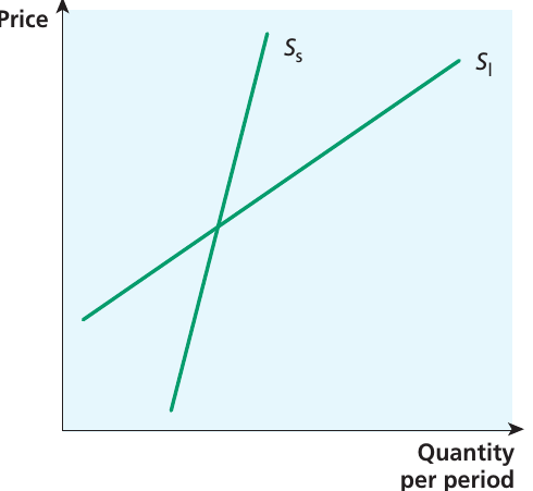
Supply elasticity differences

chatImportant

It may be more feasible for firms to change their supply decisions in the long run than in the short run. For example, if firms are operating close to the capacity of their existing plant, machinery, or factory space, they may be unable to respond to a price increase, at least in the short run.

Key principle: Supply is more elastic in the long run than in the short run.

In the short run, firms may be able to respond to price increases only in a limited way, making supply relatively inelastic. However, firms can become more flexible in the long run by installing new machinery or building new factories, allowing supply to become more elastic.

Capital and labour flexibility

When analysing the theory of the firm, economists define the short run and long run in this way, seeing the short run as a period when firms cannot vary all inputs or all factors of production, and the long run as the period when this becomes possible. In particular, it's often supposed that capital inputs are relatively difficult to vary in the short run, whereas firms may be more able to vary the amount of labour input.

An important issue is whether goods can be stored. If it's possible for firms to hold stocks of the good, this might allow them to expand sales in the short run even if it takes time to expand production. The extent to which goods can be stored depends on the nature of the good concerned and whether it's perishable or costly to store.

Two special cases

There are two limiting cases of supply elasticity that deserve attention.

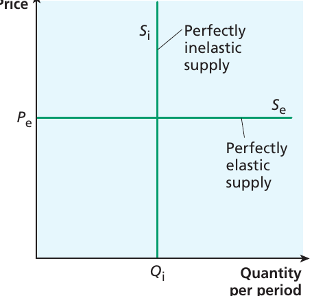
Perfectly inelastic supply

For some reason, supply may be fixed such that no matter how much the price increases, firms cannot supply any more. For example, there might be a certain amount of fish available in a market, and however high the price goes, no more can be obtained.

lightbulbExample

Example: Perfectly Inelastic Supply in Fish Markets

If fishermen know that unsold fish cannot be stored for another day, they have an incentive to sell, however low the price. In this case, there is perfectly inelastic supply.

Supply here is vertical, representing that firms will supply quantity $Q_1$ whatever the price. The price elasticity of supply is zero.

Perfectly inelastic supply: A situation in which firms can supply only a fixed quantity, so cannot increase or decrease the amount available. Elasticity of supply is zero.

Perfectly elastic supply

At the opposite extreme is perfectly elastic supply, where firms are prepared to supply any amount of the good at the going price. The supply curve is given by the horizontal line $S_e$ at price $P_e$ .

Perfectly elastic supply: A situation in which firms will supply any quantity of a good at the going price. Elasticity of supply is infinite.

Summary of PES values

PES value	Description
0	Perfectly inelastic supply
Between 0 and +1	Inelastic supply
Greater than +1	Elastic supply
Infinity	Perfectly elastic supply

chatImportant

Common Confusion Alert:

Be careful not to confuse the price elasticity of supply (PES) with the price elasticity of demand (PED), as they relate to different sides of the market and are determined by different influences.

The PES measures how producers respond to price changes
The PED measures how consumers respond to price changes

Make sure you can list the determinants of each.

Remember!

bookmarkSummary

Key Points to Remember:

Supply refers to the quantity of a good or service that firms are willing and able to sell at any given price during a specific time period
In competitive markets, firms typically supply more output at higher prices, creating an upward-sloping supply curve that reflects the positive relationship between price and quantity supplied
Changes in production costs, technology, taxes and subsidies, or the prices of related goods may cause shifts of the supply curve, with firms being prepared to sell more (or less) output at any given price
Expectations about future prices may affect current supply decisions, particularly for goods that can be stored or that take time to produce
Price elasticity of supply (PES) measures the sensitivity of quantity supplied to a change in price, and can be expected to be greater in the long run than in the short run, as firms have more flexibility to adjust their production decisions in the long run
Remember to distinguish between movements along the supply curve (caused by price changes) and shifts of the supply curve (caused by changes in other factors)

The Nature of Supply (Edexcel A-Level Economics A): Revision Notes