National Income and Macroeconomic Equilibrium (Edexcel A-Level Economics A): Revision Notes

National Income and Macroeconomic Equilibrium

Introduction

Understanding how an economy functions requires examining the relationships between income, expenditure and output. This note explores these connections through the circular flow model and examines how economies reach equilibrium through the interaction of aggregate demand and aggregate supply. We'll also investigate the multiplier effect, which explains how changes in spending can have magnified impacts on national income.

The circular flow of income, expenditure and output

The circular flow model provides a simplified framework for understanding how an economy operates. It illustrates the connections between different sectors and how resources, goods, services and money move through the economic system.

The basic circular flow model

In its simplest form, the circular flow model considers just two economic agents: households and firms. This simplified version assumes there is no government sector and no international trade.

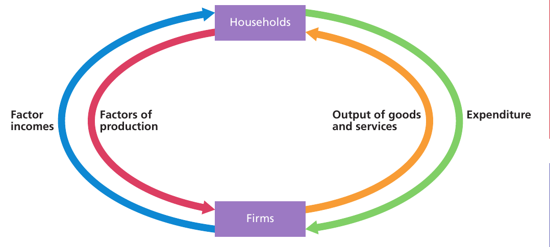
The model shows four key flows between households and firms:

• Factors of production flow from households to firms (labour, capital, land, enterprise)
• Factor incomes flow from firms to households (wages, interest, rent, profit) in return for these productive resources
• Goods and services flow from firms to households as output
• Expenditure flows from households to firms as consumers purchase goods and services

This creates a continuous loop where households supply productive resources to firms, receive income in return, then spend that income on the output produced by firms.

The three measures of economic activity

Because the circular flow represents a closed system, the flows must balance. This means economic activity can be measured in three equivalent ways:

1. Income method - measuring the total incomes paid out by firms to households (wages, salaries, interest, rent, profits)
2. Expenditure method - measuring the total spending on goods and services in the economy
3. Output method - measuring the total value of goods and services produced

What each measure tells us

Each measurement approach reveals different information about the economy's structure:

The expenditure-side estimate shows how society's resources are being allocated. It reveals what proportion is devoted to consumption, investment, government spending, and net trade (exports minus imports).

The income-side estimate provides insight into the distribution of income between different factors of production. It shows the balance between:

• Labour income (wages and salaries)
• Capital income (interest)
• Land income (rents)
• Enterprise income (normal profit)

The output-side estimate focuses on the economic structure, showing the balance between:

• Primary production (agriculture, mining)
• Secondary activity (manufacturing)
• Tertiary activity (services)

Injections and withdrawals

The simple circular flow model has limited applicability to real-world economies because it represents a closed system. In reality, money both enters and exits the circular flow through various channels.

Understanding injections and withdrawals

Withdrawals (also called leakages) represent money flowing out of the circular flow. Injections represent money flowing into the system. These arise from three sources each:

Withdrawals consist of:

• Savings (S) - household income not spent on consumer goods
• Taxation (T) - money collected by government from households and firms
• Imports (M) - spending on goods and services from abroad

Injections consist of:

• Investment (I) - spending by firms on capital goods and productive capacity
• Government spending (G) - expenditure on public goods and services
• Exports (X) - foreign spending on domestically produced goods and services

The expanded circular flow

When we incorporate injections and withdrawals, the circular flow becomes more realistic. Total expenditure now includes not just household consumption, but also investment by firms (I), government expenditure (G), and export revenues (X).

The multiplier effect

An important consequence of the circular flow is that increases in spending can trigger rounds of further expenditure. For example, when firms increase investment spending, they hire additional workers to expand production. These workers then spend their wages on consumer goods, generating income for shopkeepers and other businesses. This creates a second round of expenditure, leading to what economists call the multiplier effect.

The multiplier explains why government spending on infrastructure projects, such as road construction, can have impacts on the economy exceeding the initial expenditure.

Income and wealth

Students often confuse income and wealth, but these represent fundamentally different economic concepts.

Distribution of income and wealth

In the UK, wealth is distributed much less evenly than income. The wealthiest 10% of households hold approximately 43% of total wealth, while the least wealthy half of households hold just 9%. In contrast, the top 10% by income receive 27% of disposable income.

Wealth is strongly influenced by:

• Changes in house prices
• The value of pension funds
• Inheritance patterns

The link between wealth and income

Although wealth and income differ, they are interconnected. Inequality in wealth can generate inequality in income because wealth creates income flows. Property ownership generates rental income, while share ownership produces dividend income. These income streams flow back into household budgets, potentially widening income inequality.

Macroeconomic equilibrium

The circular flow model demonstrates that total expenditure, income and output should be equal when measured accurately. However, this doesn't mean the economy is always in equilibrium in the sense that all economic agents are satisfied with the outcome.

What is macroeconomic equilibrium?

Macroeconomic equilibrium occurs when planned expenditure equals planned output. This differs from the accounting identity that actual expenditure always equals actual output. The distinction matters because unplanned changes in inventories (stock levels) bridge the gap between planned and actual figures.

Short-run equilibrium using AD/AS analysis

To properly analyse macroeconomic equilibrium, we need to bring together aggregate demand and aggregate supply. The equilibrium position is found where these curves intersect, determining both the economy's real output level and overall price level.

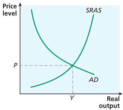
In this diagram:

• The vertical axis shows the price level
• The horizontal axis shows real output
• The SRAS (short-run aggregate supply) curve slopes upward
• The AD (aggregate demand) curve slopes downward
• Equilibrium occurs at price level P and output level Y

This represents an equilibrium because, at this price level, aggregate supply matches aggregate demand. Firms have no reason to change their behaviour in the next period, and households will continue their current spending patterns.

Changes in aggregate demand

When market conditions change, the equilibrium position shifts. Consider what happens if government expenditure increases, shifting the aggregate demand curve rightward.

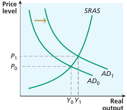
The economy moves from its initial equilibrium (with aggregate demand at AD₀) to a new equilibrium position (with aggregate demand at AD₁). This results in:

• Higher equilibrium output (Y₁ instead of Y₀)
• A higher price level (P₁ instead of P₀)

Sustainability of the new equilibrium

An important question concerns whether this new equilibrium can be sustained. Suppose the original output level Y₀ represented full employment. In the short run, firms can increase output by raising prices and employing more workers. However, they may eventually face capacity constraints - perhaps needing to pay workers overtime or hire additional office space.

The effect of a supply shock

The AD/AS model can also analyse external shocks affecting aggregate supply. For example, consider what happens when oil prices rise sharply due to supply disruptions. This increases firms' costs and reduces aggregate supply.

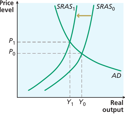
The economy begins in equilibrium with output at Y₀ and price level at P₀. The oil price increase causes the aggregate supply curve to shift from SRAS₀ to SRAS₁. After the economy adjusts to its new equilibrium:

• Real output has fallen to Y₁
• The price level has increased to P₁

Long-run equilibrium

Long-run equilibrium is analysed using the long-run aggregate supply (LRAS) curve alongside aggregate demand.

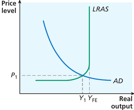
The LRAS curve shows the relationship between aggregate supply and price level in the long run. In the classical/monetarist view, the LRAS is vertical at the full employment level of output (Y_FE). This reflects the view that, in the long run, the economy naturally gravitates toward full employment regardless of the price level.

Equilibrium occurs where AD intersects LRAS. The figure shows equilibrium at:

• Price level P₁
• Full employment output Y_FE

Can equilibrium occur below full employment?

Keynesians would argue that macroeconomic equilibrium can occur at output levels below full employment. Figure 13.7 (shown in the source material) presents this view using a Keynesian LRAS curve that has both a horizontal section (at low output levels) and a vertical section (at full employment).

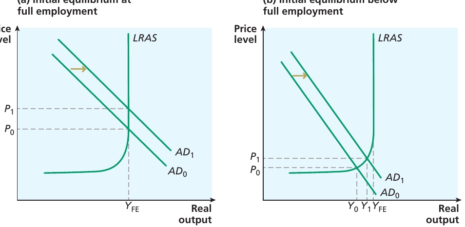
These diagrams compare two scenarios:

Panel (a): Initial equilibrium at full employment

When the economy starts at full employment (Y_FE) and aggregate demand increases (from AD₀ to AD₁), the only effect is a rise in the price level (from P₀ to P₁). Real output remains at Y_FE because the economy cannot sustainably produce beyond full employment capacity.

Panel (b): Initial equilibrium below full employment

When the economy starts below full employment, an increase in aggregate demand (from AD₀ to AD₁) has different effects. Both price level and real output increase. The economy moves closer to full employment, rising from Y₀ toward Y_FE, but may not reach it fully.

The multiplier

John Maynard Keynes identified that certain types of spending can have multiplied effects on equilibrium output through successive rounds of expenditure.

How the multiplier works

Suppose the government increases its expenditure by $1 billion, perhaps through a road-building programme. This initial spending generates income for construction workers and contractors. These workers then spend a portion of their additional income on consumer goods, creating income for shopkeepers and café owners. They, in turn, spend part of their additional income, generating a third round of spending.

This process continues through multiple rounds, with each round of spending generating the next. The total increase in equilibrium output can therefore exceed the original $1 billion increase in government spending. This is the multiplier effect.

The multiplier is defined as the ratio of the change in equilibrium real income to the autonomous change that brought it about. Mathematically:

$\text{Multiplier} = \frac{1}{\text{marginal propensity to withdraw}}$

Withdrawals and the multiplier

The size of the multiplier depends critically on withdrawals from the circular flow. These withdrawals determine how much of each round of additional income gets spent in the next round versus leaking out of the system.

Three types of withdrawal affect the multiplier:

Marginal propensity to save (mps) - the proportion of additional income that households save rather than spend.

Marginal propensity to import (mpm) - the proportion of additional income spent on imported goods and services. This spending benefits foreign producers rather than domestic firms, so it leaks from the UK circular flow.

Marginal propensity to tax (mpt) - the proportion of additional income collected by government as taxation.

Together, these determine the marginal propensity to withdraw (mpw):

$\text{mpw} = \text{mps} + \text{mpm} + \text{mpt}$

The marginal propensity to consume (mpc) represents the proportion of additional income spent on domestic goods and services:

$\text{mpc} = 1 - \text{mpw}$

Calculating the multiplier

The multiplier formula is:

$\text{multiplier} = \frac{1}{\text{mpw}}$

The formula varies depending on which sectors we include in our model:

Economic model	Multiplier formula
Closed economy with no government sector	$\frac{1}{\text{mps}}$
Open economy with no government sector	$\frac{1}{\text{mps} + \text{mpm}}$
Closed economy with government sector	$\frac{1}{\text{mps} + \text{mpt}}$
Open economy with government sector	$\frac{1}{\text{mps} + \text{mpt} + \text{mpm}} = \frac{1}{\text{mpw}}$

The multiplier and aggregate demand

The existence of the multiplier has important implications for the aggregate demand curve. When autonomous expenditure increases (such as government spending or investment by firms), the initial rightward shift of the AD curve is augmented by further shifts as successive rounds of additional expenditure work through the system.

This suggests that government spending could be a powerful tool for managing aggregate demand. However, several considerations limit this power:

1. Position relative to full employment - The closer the economy operates to full employment, the smaller the elasticity of supply. Increases in aggregate demand near full employment have larger effects on the price level and smaller effects on real output. The multiplier simply means greater upward pressure on the equilibrium price level.

2. Domestic supply flexibility - If domestic supply is inflexible and cannot meet increased demand, more of the increased income spills over into purchasing imports. This dilutes the multiplier effect.

3. Time lags - The successive rounds of spending take time to work through the economy. The full multiplier effect may not materialize for many months.