Seasonal variations Revision Notes for AQA GCSE Statistics

Seasonal variations

What are seasonal variations?

Seasonal variations are regular patterns that repeat at specific times throughout a cycle, such as yearly quarters or terms. In time series analysis, we use seasonal variations to understand how actual values differ from the general trend at predictable intervals.

For example, ice cream sales typically peak in summer and drop in winter, whilst heating costs show the opposite pattern. By identifying these seasonal patterns, businesses can make better predictions and plan more effectively.

infoNote

Seasonal patterns are everywhere in business and economics. Think about retail sales during holiday seasons, electricity usage during different weather periods, or even website traffic patterns throughout the week. Understanding these patterns helps organisations allocate resources more efficiently and set realistic targets.

Key formulas you need to know

There are three essential formulas for working with seasonal variations that form the foundation of seasonal analysis:

chatImportant

Essential Formulas for Seasonal Variation Analysis:

1. Seasonal variation at a point: $\text{Seasonal variation} = \text{Actual value} - \text{Trend value}$

2. Estimated mean seasonal variation: $\text{Estimated mean seasonal variation} = \frac{\text{Sum of all seasonal variations for that season}}{\text{Number of observations}}$

3. Predicted value: $\text{Predicted value} = \text{Trend line value} + \text{Estimated mean seasonal variation}$

These formulas work together to help you analyse patterns and make forecasts based on historical data.

Understanding the calculation process

The process of calculating seasonal variations involves several steps that build upon each other. First, you identify the actual values from your data and the corresponding trend values from your trend line. The difference between these gives you the seasonal variation for each data point.

Once you have seasonal variations for the same season across multiple cycles, you can calculate the mean seasonal variation for that particular season. This average represents the typical seasonal effect you can expect.

infoNote

Think of the trend line as showing the general direction your business is heading, while seasonal variations show the regular ups and downs that happen around that trend. The combination of both gives you a complete picture of your data's behaviour.

Worked example: football boot sales

Let's examine how seasonal variations work using real sales data from a sports shop.

lightbulbExample

Worked Example: Football Boot Sales Analysis

Table

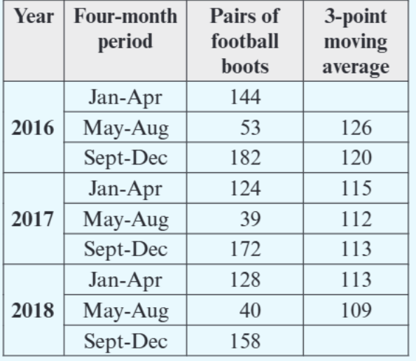
The table shows football boot sales over three years, broken down into four-month periods. Notice how sales consistently drop during May-August (summer months) and peak during other periods when football is more popular.

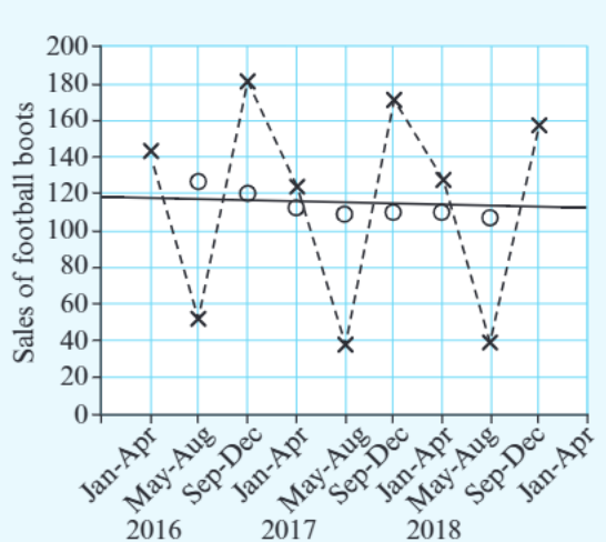
This graph clearly shows the seasonal pattern, with the jagged line (marked with X) representing actual sales and the smoother line (marked with circles) showing the trend.

Step-by-step calculation walkthrough

lightbulbExample

Worked Example: Calculating Mean Seasonal Variation

Let's calculate the seasonal variation for January-April periods using the data provided:

Table

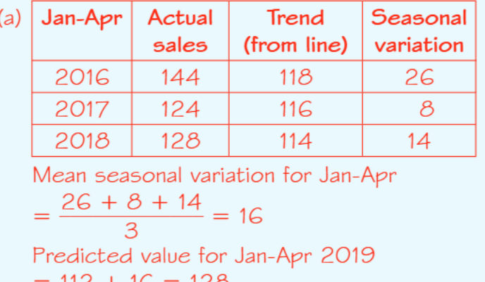
Step 1: Identify actual sales and trend values for Jan-Apr periods:

2016: Actual = 144, Trend = 118
2017: Actual = 124, Trend = 116
2018: Actual = 128, Trend = 114

Step 2: Calculate seasonal variation for each year using the formula: $\text{Seasonal variation} = \text{Actual} - \text{Trend}$

2016: $144 - 118 = 26$
2017: $124 - 116 = 8$
2018: $128 - 114 = 14$

Step 3: Calculate the mean seasonal variation for Jan-Apr: $\text{Mean} = \frac{26 + 8 + 14}{3} = \frac{48}{3} = 16$

Step 4: Make a prediction for Jan-Apr 2019: From the trend line, the trend value for 2019 is 112

$\text{Predicted value} = 112 + 16 = 128 \text{ pairs of boots}$

Making predictions using seasonal variations

Once you have calculated the mean seasonal variation for each season, you can make predictions for future periods. The key is to follow a systematic approach:

infoNote

The Prediction Process:

Extend your trend line to the future period you want to predict
Read off the trend value for that period
Add the appropriate mean seasonal variation
This gives you your predicted actual value

This method works because it combines the overall direction of the business (the trend) with the predictable seasonal effects.

Limitations and considerations

chatImportant

Critical Limitations to Remember:

While seasonal variation analysis is powerful, it has important limitations. The main concern is that trends may not continue indefinitely into the future. Economic conditions, market changes, or external factors can alter both the trend and seasonal patterns.

For this reason, predictions become less reliable the further into the future you go. It's generally more appropriate to make short-term predictions (one or two cycles ahead) rather than long-term forecasts.

Practice example: student enrolment

lightbulbExample

Practice Example: Student Enrolment Analysis

Table

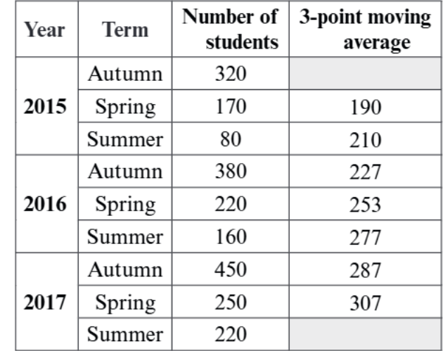
This enrolment data shows another example of seasonal variations. Notice how student numbers consistently drop during summer terms and peak during autumn terms. You could apply the same calculation process to:

Calculate seasonal variations for each term
Find mean seasonal variations by term type
Predict future enrolment numbers
Help the institution plan resources and staffing

The same principles apply whether you're analysing sales data, enrolment figures, or any other time series with seasonal patterns.

Remember!

bookmarkSummary

Key Points to Remember:

Seasonal variation = Actual value - Trend value - this measures how much a specific point differs from the general trend
Mean seasonal variation is calculated by averaging all seasonal variations for the same season across multiple cycles
Predictions combine trend and seasonal effects: Predicted value = Trend value + Mean seasonal variation
Seasonal patterns repeat cyclically - what happened in previous summers/winters tends to happen again
Don't extrapolate too far - predictions become unreliable when projecting many cycles into the future

Seasonal variations (AQA GCSE Statistics): Revision Notes