Variations in a time series (AQA GCSE Statistics): Revision Notes
Variations in a time series
When you look at a time series graph, you'll often notice that the data doesn't follow a perfectly smooth pattern. Instead, it shows various variations that make the line go up and down in different ways. Understanding these variations is crucial for interpreting what the data is actually telling us about trends and patterns over time.
Time series analysis is fundamental in many fields including economics, business forecasting, and scientific research. Learning to identify and interpret variations helps you make better predictions and understand underlying patterns in data.
What are variations in a time series?
A time series graph displays data collected over regular time periods, and these graphs commonly show variations in their patterns. These variations help us understand both the long-term direction of the data and any repeating patterns that occur.
There are two main types of variations you need to recognise:
General trend: This shows the overall direction that your data is moving in over the long term. It could be increasing (going up), decreasing (going down), or remaining relatively stable. Think of this as the "big picture" of what's happening to your data.
Seasonal variations: These are patterns that repeat themselves across regular time periods. For example, ice cream sales might be higher every summer and lower every winter - this creates a seasonal pattern that repeats each year.
Seasonal variations don't always follow calendar seasons. They can be monthly patterns (like retail sales), weekly patterns (like website traffic), or even daily patterns (like electricity usage).
How to identify variations
To properly identify variations in your time series data, you need to understand how values relate to the overall trend.
Variations are simply the differences between the actual data values and what the trend line suggests the value should be. When you draw a trend line through your data points, some actual values will sit above this line, while others will sit below it.
Here's how to interpret these differences:
- Positive variations: When actual values are higher than the trend line suggests
- Negative variations: When actual values are lower than the trend line suggests
The size of any seasonal variation equals the difference between the actual recorded value and the corresponding trend value at that point in time.
Worked example: analysing gas bill variations
Worked Example: Gas Bill Seasonal Analysis
Let's work through a practical example using quarterly gas bill data to see how variations work in practice.
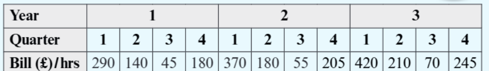
The table shows gas bill costs for each quarter over a three-year period. When we plot this data as a time series graph, we can identify both trends and seasonal patterns.
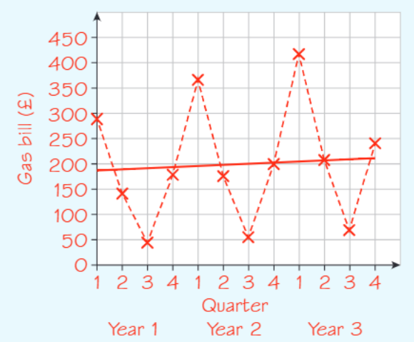
Looking at this graph, we can observe several important features:
The general trend: The overall cost of gas has been increasing year on year. This upward trend shows that gas bills are generally getting more expensive over time.
Seasonal variations: There's a clear repeating pattern where gas bills are consistently higher in quarters 1 and 4 (typically the colder months) and lower in quarters 2 and 3 (the warmer months). This makes perfect sense because people use more gas for heating during winter.
Measuring the variations: In quarters 1 and 4, the actual values sit well above the trend line, creating positive variations. In quarters 2 and 3, the actual values fall below the trend line, creating negative variations.
The reason for these seasonal variations is straightforward - more gas is needed for heating during the colder months, whilst less is required during the warmer summer period.
Key calculation method
Systematic Method for Calculating Seasonal Variations:
- Plot your time series data on a graph with appropriate scales
- Draw a trend line that shows the general direction of your data
- Identify seasonal patterns by looking for values that consistently appear above or below the trend line at regular intervals
- Calculate variation sizes by finding the difference between each actual value and its corresponding trend value
- Classify variations as positive (above trend) or negative (below trend)
Formula: Variation = Actual value - Trend value
Interpreting seasonal cycles
When you're analysing seasonal variations, look for patterns that repeat over regular time periods. Understanding these cycles is essential for business planning and forecasting.
Pattern Recognition in Seasonal Cycles
In the gas bill example, we see a clear 4-quarter (yearly) cycle where:
- Winter quarters show positive variations (higher than trend)
- Summer quarters show negative variations (lower than trend)
This type of analysis helps businesses plan for predictable changes in demand, costs, or sales throughout different seasons.
Common exam tips
Critical Exam Success Points:
- Always explain why seasonal variations occur - link them to real-world factors
- Remember that trend lines show the general direction, not the exact path of individual data points
- When describing variations, use precise mathematical language: "above/below the trend line" rather than just "high/low"
- Calculate variations as: Actual value - Trend value
- Don't forget to state whether variations are positive or negative
Remember!
Key Points to Remember:
- Time series variations come in two types: general trends and seasonal patterns
- Trend lines help you see the overall direction while highlighting seasonal variations
- Positive variations occur when actual values exceed the trend, negative variations occur when actual values fall below the trend
- Seasonal variations repeat at regular intervals and often have logical real-world explanations
- Calculate variation size by finding the difference between actual and trend values