Stock Control Problems (Leaving Cert Applied Maths): Revision Notes

Stock Control Problems

Stock control problems are a key application of dynamic programming that help businesses determine the most cost-effective way to manage their inventory and production over time. These problems involve balancing production costs, storage expenses, and demand requirements to minimise total costs.

What is a stock control problem?

A stock control problem involves deciding when and how much to produce each month to meet customer demand while minimising total costs. The challenge is finding the optimal balance between:

• Production costs - including overheads and labour
• Storage costs - for keeping items in stock
• Capacity constraints - maximum production and storage limits
• Demand requirements - orders that must be fulfilled on time

Key components and costs

Stock control problems typically involve several types of costs that must be considered when developing the optimal production strategy.

Storage costs

These are charged for each item held in stock each month. In our example, storage costs €40 per scooter per month, with a maximum storage capacity of 3 scooters.

Overhead costs

Fixed costs that occur whenever production takes place, regardless of quantity produced. These might include heating, electricity, and lighting costs - typically €200 per month when production occurs.

Hired labour costs

Additional costs incurred when production exceeds normal capacity. If production goes above 3 units per month, an assistant must be hired at an additional cost of €350.

Other variable costs

Additional costs that may vary depending on the specific situation, such as overtime or deviation costs (OVD).

The cost formula

The total cost for any production decision follows this fundamental structure:

$\text{Total Cost} = \text{Storage} + \text{Overheads} + \text{Hired Labour} + \text{OVD}$

This formula is applied to each possible production scenario to find the optimal solution.

Dynamic programming approach

Stock control problems use backwards induction - starting from the final time period and working backwards to the beginning. This approach ensures we make optimal decisions at each stage by considering all future consequences.

The backwards induction method is essential because each production decision affects not only immediate costs but also future storage requirements and production flexibility.

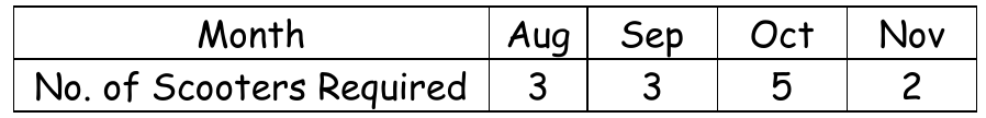
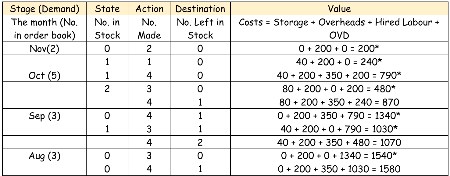
The decision table structure

Each stage of the dynamic programming solution uses a decision table with these columns:

• Stage (Demand): The time period and quantity required
• State: Number of units currently in stock
• Action: Number of units to produce
• Destination: Number of units remaining in stock after meeting demand
• Value: Total cost calculation for this decision path

Working backwards methodology

The backwards induction process follows a systematic three-step approach that guarantees optimal results.

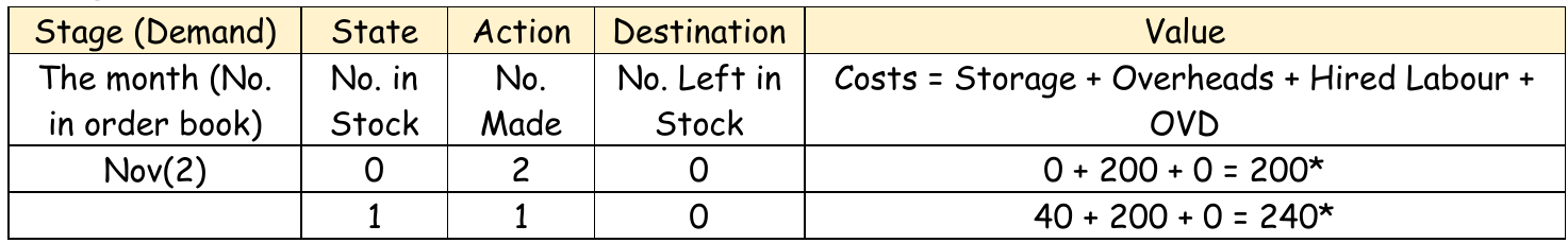
Step 1: Start with the final month

Begin with the last month in your planning period. Calculate costs for all possible starting stock levels and production decisions.

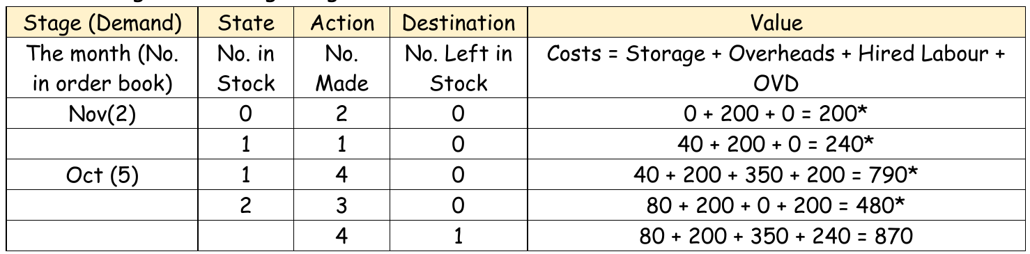
Step 2: Work backwards through each month

For each previous month, consider all possible stock levels and production options. The key insight is that the cost for any decision equals the immediate cost plus the optimal future cost.

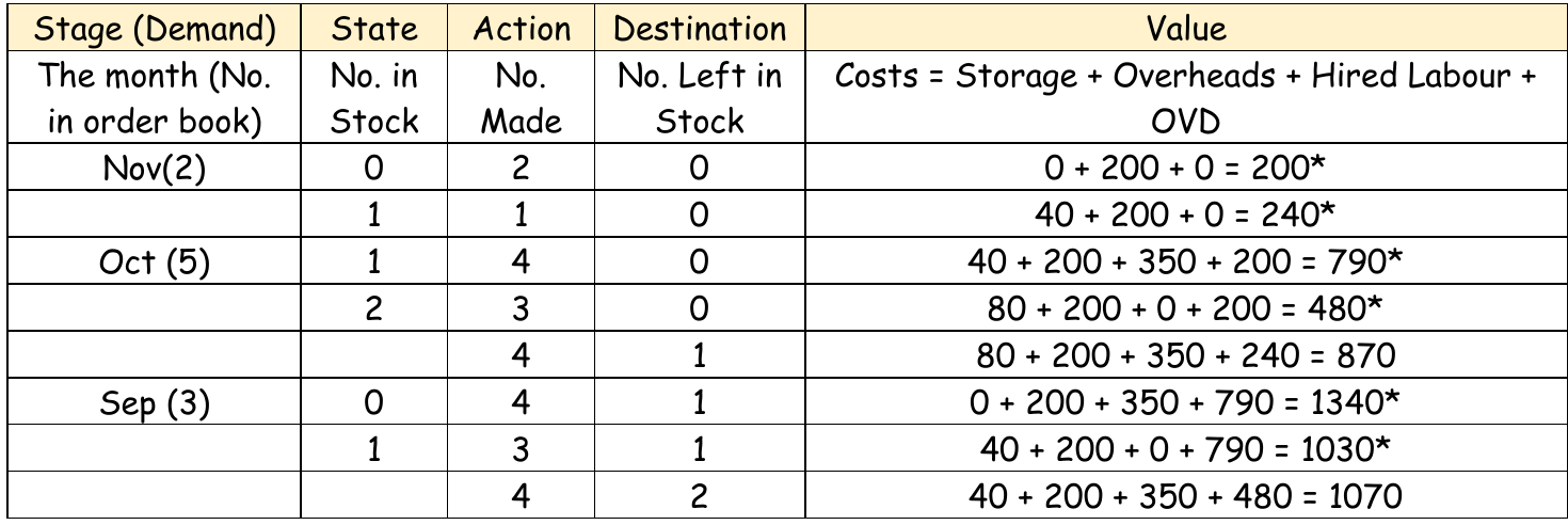
Step 3: Build the complete solution

Continue working backwards until you reach the first month. This creates a complete decision tree showing the optimal path.

Finding the optimal solution

The optimal solution is identified through a systematic evaluation process that ensures all constraints are satisfied while minimising costs.

The process involves:

1. Marking feasible options: Solutions that don't violate constraints (marked with asterisks)
2. Comparing costs: Choosing the lowest-cost option at each stage
3. Tracing the path: Following the optimal decisions from first month to last

Calculating profitability

Once you have the optimal production plan and minimum costs, you can calculate overall profitability using this comprehensive formula:

$\text{Overall Profit} = \text{Total Revenue} - \text{Total Costs} - \text{Fixed Costs}$

Where:

• $\text{Total Revenue} = (\text{Number of units sold}) \times (\text{Price per unit})$
• $\text{Total Costs} = \text{Minimum cost from dynamic programming}$
• $\text{Fixed Costs} = \text{Any additional fixed expenses like salaries}$

Exam tips

When solving stock control problems in examinations, following these strategic approaches will help ensure accuracy and completeness:

• Always work backwards from the final month
• Check that your solutions respect all constraints (production capacity, storage limits)
• Mark optimal solutions clearly in your tables
• Show all cost calculations step by step
• Don't forget to include all cost components in your formula
• Verify your final answer by checking the complete production plan