The Shape of a Distribution Revision Notes for Leaving Cert Mathematics

The Shape of a Distribution

Introduction

When we create histograms to represent data, we often notice that different datasets produce different shapes. Understanding these shapes is crucial for interpreting data correctly and choosing the right statistical measures. The shape of a distribution tells us how the data is spread out and where most values are concentrated.

Histograms are extremely useful tools because they allow us to quickly see where data lies and get a clear picture of how it's distributed. Some distributions appear balanced and symmetrical, while others are skewed in one direction or another.

infoNote

Understanding distribution shapes is fundamental to statistical analysis. The shape determines which measures of central tendency are most appropriate and helps predict patterns in real-world data.

Types of distributions

Symmetrical distributions

A symmetrical distribution has a line of symmetry running through its centre. This means that if you were to fold the histogram in half along this line, both sides would match perfectly.

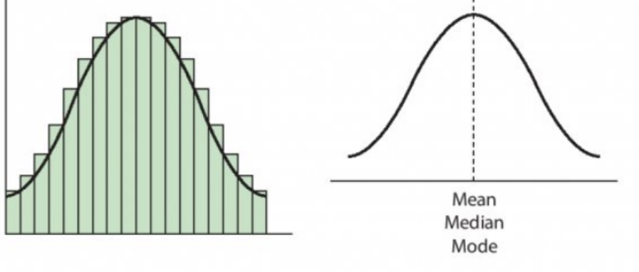
Key characteristics:

Has an axis of symmetry down the middle
Both sides of the distribution are mirror images
Creates a bell-shaped curve when drawn as a smooth line
The mean, median, and mode all have the same value
$\text{Mean} = \text{Median} = \text{Mode}$

The most important type of symmetrical distribution is called the normal distribution. This is one of the most common and significant distributions in statistics. You'll encounter normal distributions frequently in real life.

infoNote

Real-life examples of symmetrical distributions:

Heights of people in a large random sample
Intelligence quotient (IQ) scores of a population
Measurement errors in scientific experiments

Positive skew (right-skewed distributions)

A positive skew occurs when most of the data is concentrated at the lower values, with fewer observations at the higher values. This creates a long tail extending to the right of the distribution.

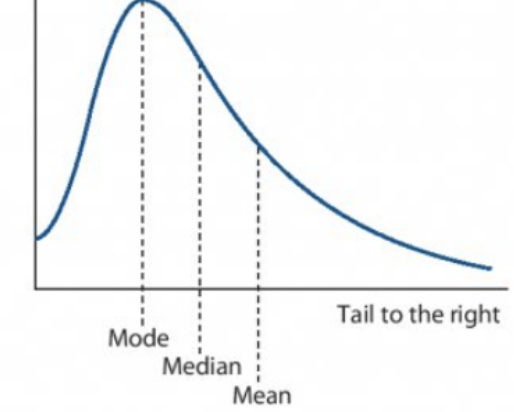
Key characteristics:

Most data clustered at lower values (left side)
Tail extends to the right
The mean is pulled towards the tail (towards higher values)
$\text{Mean} > \text{Median} > \text{Mode}$

infoNote

Memory tip: In a positive skew, most of the data is to the left, but the tail points right (positive direction).

infoNote

Real-life examples of positive skew:

Number of children in families (most have 1-3 children, few have many)
Age at which people first learn to ride a bicycle
Age at which people marry
Income distribution in most countries

Negative skew (left-skewed distributions)

A negative skew occurs when most of the data is concentrated at the higher values, with fewer observations at the lower values. This creates a long tail extending to the left of the distribution.

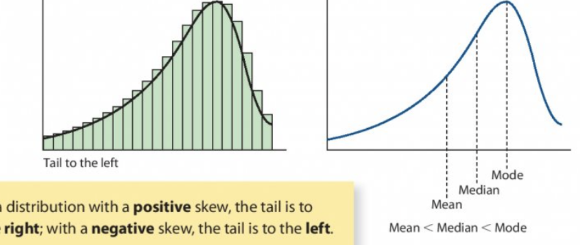
Key characteristics:

Most data clustered at higher values (right side)
Tail extends to the left
The mean is pulled towards the tail (towards lower values)
$\text{Mean} < \text{Median} < \text{Mode}$

infoNote

Memory tip: In a negative skew, the tail points left (negative direction).

infoNote

Real-life examples of negative skew:

Ages at which people get their first pair of reading glasses (most people need them later in life)
Heights of basketball players (most are tall, few are short)
Exam scores when most students perform well

Relationship between mean, median and mode

Understanding how the mean, median, and mode relate to each other helps identify the type of distribution:

Distribution Type	Relationship	Explanation
Symmetrical	$\text{Mean} = \text{Median} = \text{Mode}$	All measures coincide at the centre
Positive skew	$\text{Mean} > \text{Median} > \text{Mode}$	Mean pulled right by the tail
Negative skew	$\text{Mean} < \text{Median} < \text{Mode}$	Mean pulled left by the tail

chatImportant

The mean is always pulled in the direction of the skew because it's affected by extreme values in the tail. The median is less affected, and the mode represents the peak of the distribution.

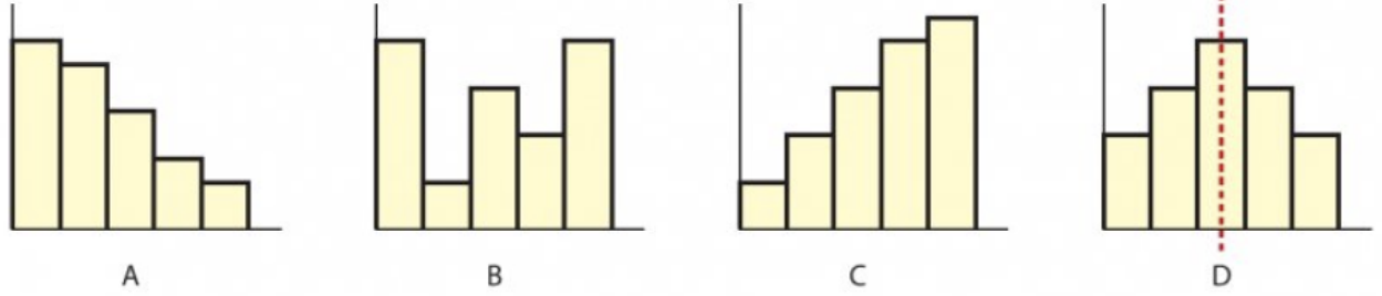
How to identify distribution shapes

lightbulbExample

Step-by-Step Guide: Identifying Distribution Shapes

Step 1: Look for symmetry - Draw an imaginary line down the centre. Do both sides match?

Step 2: Find the peak - Where is the highest point (mode) located?

Step 3: Check for tails - Does one side extend much further than the other?

Step 4: Identify tail direction - If there's a long tail, which way does it point?

infoNote

Quick identification guide:

Bell-shaped and balanced → Symmetrical (normal)
Peak on left, tail on right → Positive skew
Peak on right, tail on left → Negative skew

Exam tips

chatImportant

Essential exam strategies:

Always state the direction of skew clearly: "positive skew" or "right skew" (both are correct)
Remember the tail rule: The skew is named after the direction the tail points
Use the mean-median-mode relationships to check your identification
Give real-life examples when asked - they demonstrate understanding
Look carefully at histogram scales - don't just count bars, consider their heights
In exam questions, explain your reasoning - don't just name the distribution type

chatImportant

Common mistakes to avoid:

Confusing positive and negative skew directions
Forgetting that the mean follows the tail
Mixing up which measure of central tendency is most affected by skew
Not considering the scale when interpreting histograms

bookmarkSummary

Key Points to Remember:

Symmetrical distributions have a line of symmetry with $\text{Mean} = \text{Median} = \text{Mode}$ , commonly seen in heights and IQ scores
Positive skew has most data at lower values with a tail to the right, where $\text{Mean} > \text{Median} > \text{Mode}$
Negative skew has most data at higher values with a tail to the left, where $\text{Mean} < \text{Median} < \text{Mode}$
The mean always chases the tail - it gets pulled in the direction of the skew due to extreme values
"Tail tells the tale" - the direction of the longest tail determines the type of skew

The Shape of a Distribution (Leaving Cert Mathematics): Revision Notes