Description of Motion (Grade 10 NSC Matric Physical Sciences): Revision Notes
Description of Motion
Motion can be described in three different ways to help us understand how objects move. These methods give us different but related information about the same motion.
Understanding motion description is fundamental to physics. Each method provides unique insights:
- Words help us conceptualize and communicate about motion
- Diagrams provide visual understanding of spatial relationships
- Graphs offer precise mathematical analysis of motion patterns
Three methods for describing motion
- Words - Using descriptive language to explain movement
- Diagrams - Visual representations showing position changes
- Graphs - Mathematical plots showing relationships between quantities
We will examine three fundamental types of motion:
- Stationary object - when the object is not moving
- Uniform motion - when the object moves at constant velocity
- Motion at constant acceleration - when the object's velocity changes at a constant rate
Key definition: instantaneous speed
Instantaneous speed is the magnitude of instantaneous velocity. This means it has the same numerical value as velocity but no direction.
Critical Distinction:
- Speed is a scalar quantity (magnitude only, no direction)
- Velocity is a vector quantity (has both magnitude and direction)
This difference is essential for physics problem-solving!
- Quantity: Instantaneous speed (v)
- Unit: metres per second (m·s⁻¹)
Stationary object
A stationary object does not move, so its position does not change over time. This is the simplest type of motion to understand.
Characteristics of a stationary object
- Position remains constant
- Displacement is zero (since position doesn't change)
- Velocity is zero (since displacement is zero)
- Acceleration is zero (since velocity is not changing)
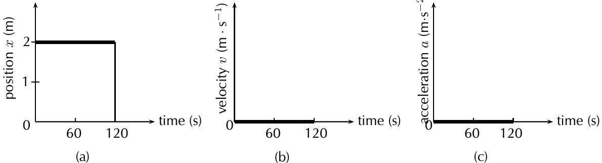
The graphs above show the motion characteristics for a stationary object. Notice that:
- Position vs time: Horizontal line showing constant position
- Velocity vs time: Horizontal line at zero
- Acceleration vs time: Horizontal line at zero
Worked Example: Vivian at the stop sign
Consider Vivian waiting for a taxi. She stands 2 metres from a stop sign at t = 0 s. After 60 s and 120 s, she is still 2 metres from the stop sign.
Analysis:
- Her position has not changed → Position = constant
- Her displacement is zero → Δx = 0
- Her velocity is zero → v = 0 m·s⁻¹
- Her acceleration is zero → a = 0 m·s⁻²
Understanding gradients in motion graphs
Gradient is a key concept for understanding motion graphs. From mathematics, we know:
Gradient (m) = change in y-value ÷ change in x-value =
Essential Gradient Relationships in Physics:
These relationships form the foundation of kinematic analysis:
- Gradient of position vs time graph = velocity
- Gradient of velocity vs time graph = acceleration
- Area under velocity vs time graph = displacement
For a stationary object, all gradients are zero because nothing is changing.
Motion at constant velocity (uniform motion)
Uniform motion means the position of an object changes at the same rate over time. The object moves with constant velocity.
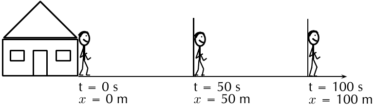
This diagram shows uniform motion - equal distances covered in equal time intervals.
Characteristics of uniform motion
- Position increases (or decreases) linearly with time
- Velocity remains constant (not changing)
- Acceleration is zero (since velocity is constant)
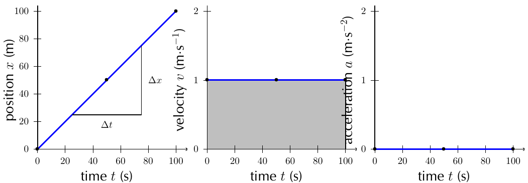
The graphs show distinctive patterns for uniform motion:
- Position vs time: Straight diagonal line (linear relationship)
- Velocity vs time: Horizontal line showing constant velocity
- Acceleration vs time: Horizontal line at zero
Calculating velocity from position graphs
For uniform motion, we can calculate velocity using the fundamental kinematic equation:
Where:
- = velocity
- = change in position
- = change in time
- = final position, = initial position
- = final time, = initial time
Motion with negative velocity
Objects can also move with constant velocity in the negative direction.
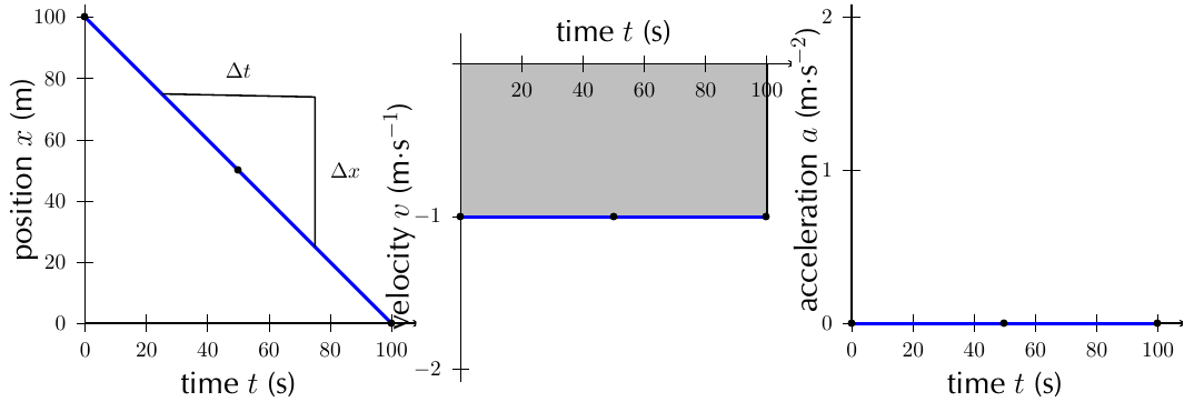
These graphs show motion with constant negative velocity:
- Position decreases linearly (downward sloping line)
- Velocity is constant but negative
- Acceleration remains zero
Direction Matters!
Negative velocity simply means motion in the opposite direction to the chosen positive direction. The object is still moving with constant speed - just in the negative direction.
Motion at constant acceleration
The final type of motion occurs when an object has constant acceleration. This means the velocity changes at a constant rate.
Understanding constant acceleration
When acceleration is constant, several important patterns emerge:
- Velocity changes by the same amount in each equal time interval
- Position changes follow a curved (parabolic) pattern
- Acceleration remains constant (horizontal line on acceleration graph)
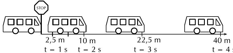
This diagram shows a bus accelerating from rest. Notice how the distances covered increase: 2.5 m, then 10 m, then 22.5 m, then 40 m in equal time intervals.
Calculating velocities during acceleration
To find velocity at different times, we calculate the gradient of position vs time at those points:
Worked Example: Bus Acceleration Velocities
For the bus example shown above:
Step 1: Calculate velocity for each time interval
- At t = 1-2 s:
- At t = 2-3 s:
- At t = 3-4 s:
Notice: Velocity increases by 5 m·s⁻¹ each second - constant acceleration!
Calculating acceleration
The fundamental equation for acceleration is:
For constant acceleration:
Using our bus example:
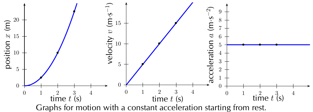
These graphs show motion with constant acceleration starting from rest:
- Position: Curved (parabolic) line
- Velocity: Straight diagonal line
- Acceleration: Horizontal line showing constant acceleration
Summary of motion graphs
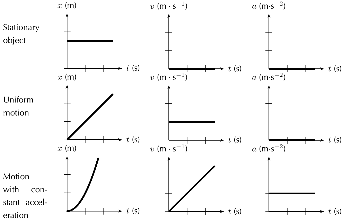
This comprehensive comparison shows the distinctive graph shapes for all three types of motion:
Key Graph Patterns to Remember:
| Motion Type | Position vs Time | Velocity vs Time | Acceleration vs Time |
|---|---|---|---|
| Stationary | Horizontal line | Zero (horizontal at x-axis) | Zero (horizontal at x-axis) |
| Uniform motion | Diagonal line | Horizontal line | Zero (horizontal at x-axis) |
| Constant acceleration | Curved line | Diagonal line | Horizontal line |
Memory Aid: Each graph type moves from simple (stationary) to more complex (accelerated) patterns.
Using area under graphs
For velocity vs time graphs, the area under the curve equals displacement:
- Rectangle area = length × width = velocity × time = displacement
- Triangle area = ½ × base × height = ½ × time × velocity change
- Total displacement = sum of all areas (considering positive/negative directions)
Area Calculation Tips:
- Break complex shapes into simple rectangles and triangles
- Always consider the sign (positive/negative) of each area
- Areas above the time axis are positive displacement
- Areas below the time axis are negative displacement
Practical investigation: motion at constant velocity
Aim
To measure position and time during motion at constant velocity and determine average velocity from a "Position vs Time" graph.
Method
The experimental procedure involves systematic measurement and analysis:
- Time a battery-operated toy car as it travels different distances
- Record measurements in a data table
- Repeat measurements and calculate averages
- Plot a "Distance vs Time" graph
- Find the gradient - this gives the average velocity
| Distance (m) | Time (s) | ||
|---|---|---|---|
| 1 | 2 | Ave. | |
| 0 | |||
| 0.5 | |||
| 1.0 | |||
| 1.5 | |||
| 2.0 | |||
| 2.5 | |||
| 3.0 |
Key observations
- Constant velocity produces a straight line graph
- Steeper gradient = faster velocity
- Gradient = rise/run = distance/time = velocity
Worked example: interpreting position-time graphs
Worked Example: Multi-Phase Motion Analysis
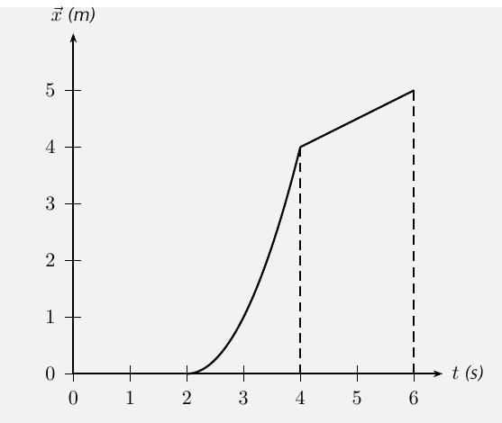
Question: Describe the motion shown in this position vs time graph.
Step 1: Identify the phases The graph shows three distinct phases based on the curve shapes.
Step 2: Analyze each phase
- 0-2 seconds: Object is stationary (horizontal line at zero position)
- 2-4 seconds: Object accelerates (curved line showing increasing position)
- 4-6 seconds: Object moves with constant velocity (straight diagonal line)
Step 3: Verify with velocity graph
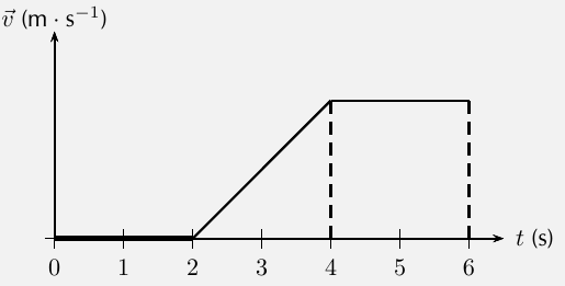
The corresponding velocity vs time graph confirms:
- Zero velocity for first 2 seconds
- Increasing velocity from 2-4 seconds (acceleration phase)
- Constant velocity from 4-6 seconds
Step 4: Check acceleration
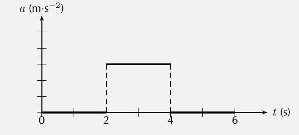
The acceleration vs time graph shows:
- Zero acceleration for 0-2 seconds and 4-6 seconds
- Constant positive acceleration from 2-4 seconds
Exam tips for motion graphs
Essential Exam Strategy Points:
-
Always check units on graph axes - marks are often lost here!
-
Identify motion type from graph shape:
- Horizontal = constant/stationary
- Diagonal = linear change
- Curved = accelerated motion
-
Calculate gradients carefully:
- Choose clear points on the line
- Show working: gradient =
- Include correct units
-
For area calculations:
- Break complex shapes into triangles and rectangles
- Consider positive/negative directions
- Show each calculation step
-
Common mistakes to avoid:
- Confusing distance with displacement
- Forgetting that speed has no direction
- Mixing up which graph gives which information
Critical Relationships to Memorize:
- Position vs time gradient = velocity
- Velocity vs time gradient = acceleration
- Area under velocity vs time graph = displacement
These three relationships are the foundation of all kinematic graph analysis!
Remember!
The three types of motion have distinct characteristics:
- Stationary objects have zero velocity and acceleration
- Uniform motion has constant velocity and zero acceleration
- Constant acceleration produces curved position graphs and linear velocity graphs
Master these patterns and you'll excel at interpreting any motion graph!