Relative Frequency Revision Notes for HSC SSCE Mathematics Advanced

Relative Frequency

Introduction to relative frequency

Relative frequency is a fundamental concept that connects experimental data to theoretical probability. When we conduct an experiment multiple times and record the outcomes, the relative frequency of each outcome provides an estimate of its true probability. This connection between data and probability theory is essential for understanding both discrete and continuous probability distributions.

A relative frequency is calculated by dividing the frequency of an outcome by the total number of trials:

$f_r = \frac{f}{n}$

where $f$ is the frequency of the outcome and $n$ is the total number of trials.

infoNote

Relative frequencies are often called experimental probabilities because they estimate the theoretical probabilities based on actual experimental results. As the number of trials increases, the relative frequencies typically become closer to the true theoretical probabilities, assuming the experiment is unbiased.

Review of mean and variance for discrete distributions

Before working with relative frequencies, let's review how to calculate the mean and variance of a discrete probability distribution.

Expected value and variance definitions

For a discrete random variable $X$ with probability function $p(x) = P(X = x)$ , the expected value or mean is:

$\mu = E(X) = \sum x \cdot p(x)$

This is the weighted average of all possible values, where each value is weighted by its probability.

The variance measures how spread out the distribution is. It is the expected value of the squared deviation from the mean:

$\text{Var}(X) = E((X - \mu)^2) = \sum (x - \mu)^2 \cdot p(x)$

There is an alternative formula for variance that is often more convenient, especially when the mean is not a whole number:

$\text{Var}(X) = E(X^2) - \mu^2 = \sum x^2 \cdot p(x) - \mu^2$

The standard deviation is simply:

$\sigma = \sqrt{\text{Var}(X)}$

Worked example: tossing four coins

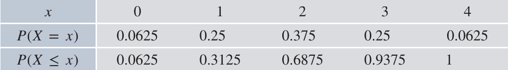
Consider the experiment of tossing four coins and counting the number of heads. The possible outcomes are 0, 1, 2, 3, or 4 heads, with theoretical probabilities shown below.

lightbulbExample

Worked Example: Method A - Using the definition $E((X - \mu)^2)$

This method calculates variance directly from the definition by finding the deviation of each value from the mean, squaring it, and taking the weighted average.

Table

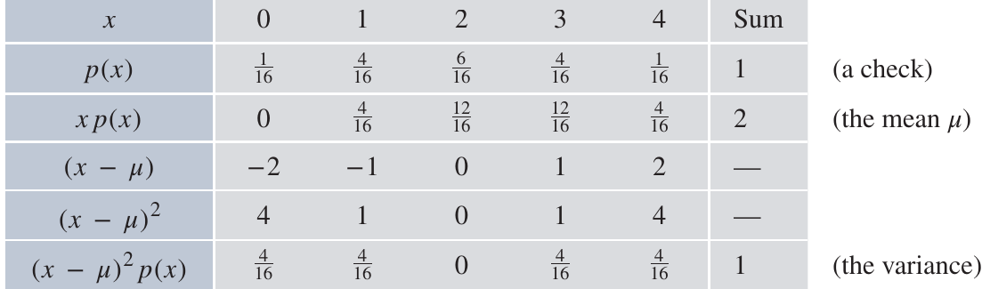
From this table:

The mean is $\mu = 2$
The variance is $\sigma^2 = 1$
The standard deviation is $\sigma = 1$

lightbulbExample

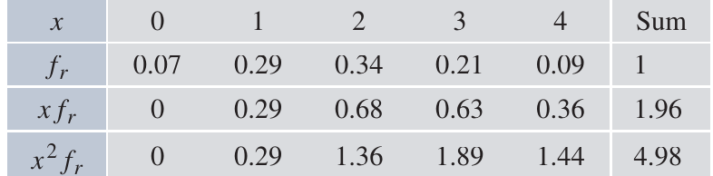
Worked Example: Method B - Using the formula $E(X^2) - \mu^2$

This alternative method is often simpler, particularly when the mean is not a whole number.

Table

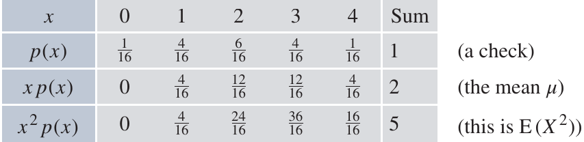
From this table:

The mean is $\mu = 2$ (from the third row)
$E(X^2) = 5$ (from the fourth row)
The variance is $\sigma^2 = E(X^2) - \mu^2 = 5 - 2^2 = 1$
The standard deviation is $\sigma = 1$

infoNote

Both methods give the same result, but Method B often involves simpler calculations, especially when dealing with non-integer means.

Cumulative distribution function

The cumulative distribution function (CDF), denoted $F(x)$ , gives the probability that the random variable is less than or equal to a particular value:

$F(x) = P(X \leq x)$

For our four-coin example, the CDF is calculated by adding up all probabilities up to and including each value:

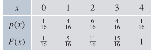
For example:

$F(3) = p(0) + p(1) + p(2) + p(3) = \frac{1}{16} + \frac{4}{16} + \frac{6}{16} + \frac{4}{16} = \frac{15}{16}$

infoNote

The cumulative distribution function always increases from 0 to 1 as we move through all possible values. This monotonic increase is a key property of all CDFs.

Working with relative frequencies from data

Now let's see how relative frequencies connect experimental data to theoretical probabilities. Suppose we actually performed the four-coin experiment 100 times and recorded these results:

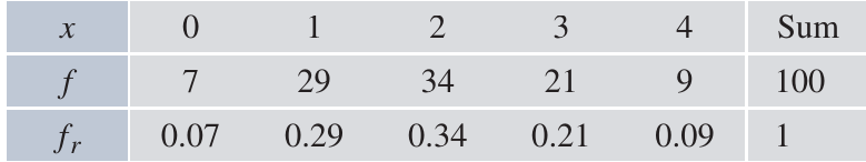
The table shows:

Values ( $x$ ): The number of heads (0, 1, 2, 3, or 4)
Frequencies ( $f$ ): How many times each outcome occurred in 100 trials
Relative frequencies ( $f_r$ ): The frequency divided by 100

chatImportant

Note that the relative frequencies sum to 1, just like theoretical probabilities. This is always true regardless of the number of trials, making relative frequencies directly comparable to probabilities.

Calculating sample statistics

We can calculate the sample mean and sample variance from relative frequencies using formulas analogous to those for theoretical distributions:

lightbulbExample

Worked Example: Calculating Sample Statistics

Sample mean:

$\bar{x} = \sum x \cdot f_r = 1.96$

Sample variance:

s^2 = \sum x^2 \cdot f_r - \bar{x}^2 \\ s^2 = 4.98 - (1.96)^2 \\ s^2 \approx 1.14

(Compare with the theoretical variance $\sigma^2 = 1$ )

Sample standard deviation:

$s = \sqrt{s^2} \approx 1.07 \text{ heads}$

(Compare with the theoretical standard deviation $\sigma = 1$ )

These sample statistics from our 100 trials are estimates of the true theoretical values. They are close but not identical to the theoretical mean of 2 and variance of 1.

Cumulative relative frequencies

Just as we can create a cumulative distribution function from probabilities, we can calculate cumulative relative frequencies from data:

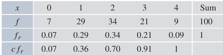
The cumulative relative frequency at each value represents the proportion of observations less than or equal to that value. For example, $\text{cf}_r = 0.70$ at $x = 2$ means that 70% of the trials resulted in 2 or fewer heads.

infoNote

These cumulative relative frequencies estimate the values of the cumulative distribution function $F(x)$ . With more trials, these estimates become more accurate.

Histograms and polygons using relative frequencies

Visual representations help us understand probability distributions and compare them with data.

Relative frequency histogram

A relative frequency histogram displays the relative frequencies as rectangular bars. When we overlay this with the theoretical distribution, we can see how well the data matches theory:

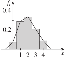
The smooth curve represents the theoretical probability distribution, while the bars show the actual relative frequencies from our 100 trials.

chatImportant

Important property: When the bars have width 1, the total area of the histogram equals 1, because the sum of all relative frequencies (or probabilities) is 1. This property connects probability to area, which becomes crucial for continuous distributions.

Cumulative relative frequency histogram

The cumulative relative frequencies can also be displayed graphically:

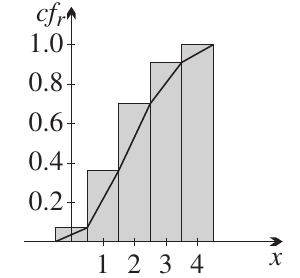
The bars increase in height because each bar represents the accumulation of all relative frequencies up to that point. The diagonal line shows how the cumulative distribution increases from 0 to 1.

Comparing theoretical and experimental distributions

When we know the theoretical probabilities, we can create the same visualisations and compare them directly with our experimental data:

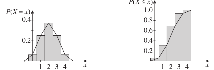
The left graph shows the probability mass function (PMF), which gives $P(X = x)$ for each value. The right graph shows the cumulative distribution function (CDF), which gives $P(X \leq x)$ .

infoNote

Notice that probability estimates from data are rarely exactly the same as theoretical probabilities due to random variation in the experimental trials. This is expected and natural.

Grouped data from continuous random variables

When working with continuous random variables, or when discrete variables have many possible values, we need to group the data into intervals called classes.

Example: heights of 100 people

Consider the heights of 100 people, measured in centimetres. Because height is continuous, we group the data into 10 cm intervals:

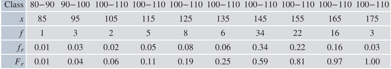
In this table:

Class: The interval of heights (e.g., 80-90 cm, 90-100 cm)
$x$ : The class centre (midpoint of each interval)
$f$ : The frequency (number of people in each interval)
$f_r$ : The relative frequency
$F_r$ : The cumulative relative frequency

Visualising grouped data

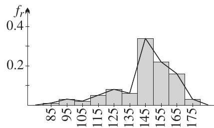
Relative frequency histogram:

Cumulative relative frequency histogram:

infoNote

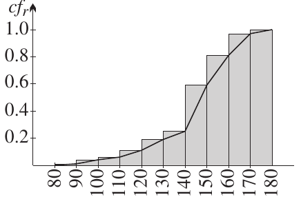
These graphs show how the data is distributed across the height intervals. The bell-shaped curve in the relative frequency histogram suggests the data may follow a normal distribution.

Deciles and percentiles

Just as quartiles divide the data into four equal parts, we can use deciles and percentiles to divide data into finer divisions.

Reading from cumulative frequency graphs

Using the cumulative relative frequency graph, we can find:

Deciles: These divide the data into ten equal parts

To find the 3rd decile, draw a horizontal line at height 0.3
To find the 7th decile, draw a horizontal line at height 0.7

Percentiles: These divide the data into one hundred equal parts

To find the 68th percentile, draw a horizontal line at height 0.68
To find the 95th percentile, draw a horizontal line at height 0.95

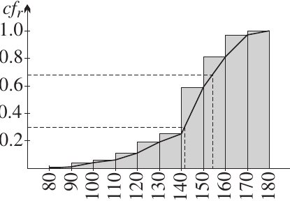
From the graph shown, the 3rd decile is approximately 142 and the 68th percentile is approximately 154.

infoNote

This graphical method may give slightly different results from other calculation methods, but it fits well with the integral-based approach used for continuous distributions.

When does a discrete distribution look continuous?

As the number of possible values in a discrete distribution increases, the graph may begin to suggest an underlying continuous curve.

Example: tossing 20 coins

When we toss 20 coins and count the heads, we get 21 possible outcomes (0 to 20 heads). The probability distribution looks like this:

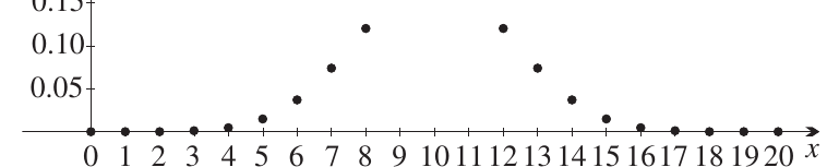
The dots suggest a smooth, bell-shaped curve. As the number of coins increases further, calculating exact probabilities becomes increasingly difficult.

chatImportant

This motivates approximating discrete distributions with continuous distributions, which is one reason continuous distributions are so useful in statistics. Continuous approximations greatly simplify calculations for large numbers of trials.

Probability and area

A key concept in continuous probability distributions is the connection between probability and area. Here's a simple example that illustrates this principle.

lightbulbExample

Worked Example: The Wandering Chook

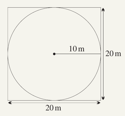
Problem: A point-chook is wandering randomly around a 20 m × 20 m square enclosure. It is equally likely to be at any location in the enclosure. A circle of radius 10 metres has been inscribed in the square. What is the probability that the chook is inside the circle?

Solution:

Area of square enclosure $= 20^2 = 400 \text{ m}^2$

Area of circle $= \pi r^2 = \pi \times 10^2 = 100\pi \text{ m}^2$

Since the chook is equally likely to be anywhere in the enclosure:

$P(\text{chook is inside circle}) = \frac{\text{area of circle}}{\text{area of square}}$

$P(\text{chook is inside circle}) = \frac{100\pi}{400} = \frac{\pi}{4} \approx 0.785$

chatImportant

This problem demonstrates how probability can be calculated using area when dealing with continuous spaces. The answer $\frac{\pi}{4}$ is not even a rational number, which shows we're beyond discrete sample spaces. This area-based approach is fundamental to continuous probability distributions.

Remember!

bookmarkSummary

Key Points to Remember:

Relative frequency is calculated by dividing frequency by total number of trials: $f_r = \frac{f}{n}$
Relative frequencies are estimates of probabilities and are often called experimental probabilities
The cumulative distribution function $F(x) = P(X \leq x)$ gives the probability of obtaining a value less than or equal to $x$
For histograms with bars of width 1, the total area equals 1 when using relative frequencies or probabilities
Cumulative relative frequencies estimate the cumulative distribution function from data
For continuous distributions, probability is associated with area rather than discrete sample spaces
As discrete distributions involve more values, they begin to resemble continuous curves, motivating the use of continuous approximations

Relative Frequency (HSC SSCE Mathematics Advanced): Revision Notes