Systematic Curve Sketching with the Derivative Revision Notes for HSC SSCE Mathematics Advanced

Systematic Curve Sketching with the Derivative

Introduction to systematic curve sketching

When sketching unfamiliar curves, we can use a systematic approach that combines earlier non-calculus methods with calculus techniques. Previously, we used a four-step approach focusing on domain, symmetry, intercepts and asymptotes. Now we extend this by adding derivative analysis to examine gradient, concavity, turning points and inflections.

Most functions don't require all seven steps shown below. Typically, you'll be guided on which methods are most relevant for a particular function.

infoNote

This systematic approach has limitations - for example, it only detects symmetry about the y-axis, and doesn't account for periodic behaviour in trigonometric functions.

The seven-step systematic method

This comprehensive approach combines non-calculus and calculus techniques:

Step 1: Domain

Determine where the function is defined.

Find all x-values for which $f(x)$ exists. Always do this step first, as it affects all subsequent analysis. Look for:

Values that make denominators zero
Values that create negative numbers under even roots
Values outside the domain of inverse trigonometric functions

Step 2: Symmetry

Test whether the function is even, odd, or neither.

A function is even if $f(-x) = f(x)$ for all x in the domain (symmetric about the y-axis)
A function is odd if $f(-x) = -f(x)$ for all x in the domain (symmetric about the origin)
Most functions are neither even nor odd

Understanding symmetry can reduce the work needed in later steps.

Step 3: Intercepts and sign

Part A: Find where the curve crosses the axes

y-intercept: Substitute $x = 0$ into the function
x-intercepts (zeroes): Solve $f(x) = 0$

Part B: Determine where the function is positive and negative

Create a table of test values. Select x-values in each interval created by the x-intercepts and discontinuities, then evaluate $f(x)$ to determine the sign in each region.

This tells you which parts of the curve are above the x-axis (positive) and which are below (negative).

Step 4: Asymptotes

Part A: Vertical asymptotes

Check each discontinuity (where the function is undefined). If $f(x) \to \pm\infty$ as x approaches the discontinuity from either side, there's a vertical asymptote at that x-value.

Part B: Horizontal asymptotes

Examine what happens to $f(x)$ as:

$x \to \infty$ (right-hand behaviour)
$x \to -\infty$ (left-hand behaviour)

If $f(x)$ approaches a constant value L, then $y = L$ is a horizontal asymptote.

Step 5: The first derivative

Part A: Find critical points

Calculate $f'(x)$ , then find:

Where $f'(x) = 0$ (stationary points)
Where $f'(x)$ is undefined (potential corners or cusps)

Part B: Analyse gradient throughout the domain

Create a table of slopes by testing values of $f'(x)$ in intervals between critical points:

Where $f'(x) > 0$ : function is increasing (/)
Where $f'(x) = 0$ : stationary point (—)
Where $f'(x) < 0$ : function is decreasing ()

This analysis reveals:

Whether stationary points are maxima, minima, or horizontal inflections
Intervals where the function rises or falls

chatImportant

Common Mistake: Points where the derivative is undefined are NOT stationary points. Stationary points occur only where $f'(x) = 0$ .

Step 6: The second derivative

Part A: Find potential inflection points

Calculate $f''(x)$ , then find:

Where $f''(x) = 0$ (possible inflection points)
Where $f''(x)$ is undefined

Part B: Analyse concavity throughout the domain

Create a table of concavity by testing values of $f''(x)$ :

Where $f''(x) > 0$ : curve is concave up (∪)
Where $f''(x) = 0$ : possible inflection point
Where $f''(x) < 0$ : curve is concave down (∩)

An inflection point occurs where concavity changes (where $f''(x)$ changes sign).

Step 7: Any other features

Be aware that this systematic method doesn't capture all important features:

Axes of symmetry that aren't the y-axis
Periodic behaviour in trigonometric functions
Other special characteristics specific to certain function types

Worked example: A curve with turning points and asymptotes

lightbulbExample

Worked Example: Analysing a Rational Function with Asymptotes

Let's apply this systematic approach to a rational function that has multiple asymptotes and a turning point. This example demonstrates how calculus and non-calculus methods work together.

Consider the curve $y = \frac{1}{x(x-4)}$ .

Part a: Domain

The function is undefined where the denominator equals zero.

Setting $x(x-4) = 0$ :

$x = 0$ or $x = 4$

Domain: all real numbers except $x = 0$ and $x = 4$

In interval notation: $(-\infty, 0) \cup (0, 4) \cup (4, \infty)$

Part b: Sign analysis

The function never equals zero (the numerator is always 1), and has discontinuities at $x = 0$ and $x = 4$ .

We test values in each interval:

$x$	$-1$	$0$	$2$	$4$	$5$
$y$	$\frac{1}{5}$	*	$-\frac{1}{4}$	*	$\frac{1}{5}$

The asterisks (*) indicate discontinuities where the function is undefined.

Conclusion:

$y > 0$ (positive) when $x < 0$ or $x > 4$
$y < 0$ (negative) when $0 < x < 4$

Part c: Asymptotes

Vertical asymptotes:

At the discontinuities $x = 0$ and $x = 4$ , the function approaches infinity, so there are vertical asymptotes at these values.

Horizontal asymptote:

As $x \to \infty$ : the denominator grows much faster than the numerator, so $y \to 0$

As $x \to -\infty$ : similarly, $y \to 0$

Therefore, the x-axis ( $y = 0$ ) is a horizontal asymptote.

Part d: Finding the derivative

To find $y'$ , we use the chain rule.

Let $u = x^2 - 4x$

Then $y = \frac{1}{u}$

Therefore:

$\frac{du}{dx} = 2x - 4$

$\frac{dy}{du} = -\frac{1}{u^2}$

By the chain rule:

$y' = \frac{dy}{du} \times \frac{du}{dx}$

$y' = -\frac{1}{(x^2-4x)^2} \times (2x-4)$

$y' = -\frac{1}{x^2(x-4)^2} \times 2(x-2)$

$y' = \frac{-2(x-2)}{x^2(x-4)^2}$

$y' = \frac{2(2-x)}{x^2(x-4)^2}$

Part e: First derivative analysis

The derivative $y' = \frac{2(2-x)}{x^2(x-4)^2}$ has:

Zero at $x = 2$ (numerator equals zero)
Discontinuities at $x = 0$ and $x = 4$ (denominator equals zero)

We test values in each interval:

$x$	$-1$	$0$	$1$	$2$	$3$	$4$	$5$
$y'$	$\frac{6}{25}$	*	$\frac{2}{9}$	$0$	$-\frac{2}{9}$	*	$-\frac{6}{25}$
slope	/	*	/	—	\	*	\

Where:

/ indicates increasing (positive gradient)
— indicates stationary point (zero gradient)
\ indicates decreasing (negative gradient)
- indicates discontinuity

Interpretation:

At $x = 2$ : $y = \frac{1}{2(2-4)} = \frac{1}{2(-2)} = -\frac{1}{4}$

Since the gradient changes from positive to zero to negative, there is a maximum turning point at $(2, -\frac{1}{4})$ .

The function is:

Increasing for $x < 2$ (except at $x = 0$ where it's undefined)
Decreasing for $x > 2$ (except at $x = 4$ where it's undefined)

Part f: Sketch and range

The complete sketch shows:

Vertical asymptotes at $x = 0$ (the y-axis) and $x = 4$ (shown as dashed lines)
Horizontal asymptote at $y = 0$ (the x-axis)
Maximum turning point at $(2, -\frac{1}{4})$
Function approaching $+\infty$ as x approaches 0 from the left and as x approaches 4 from the right
Function approaching $-\infty$ as x approaches 0 from the right and as x approaches 4 from the left

From the graph, we can see the function takes all positive values above the horizontal asymptote, and all negative values at or below the maximum's y-coordinate.

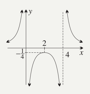
Range: $y > 0$ or $y \leq -\frac{1}{4}$

In interval notation: $\left(-\infty, -\frac{1}{4}\right] \cup (0, \infty)$

Exam tips

infoNote

Key Strategies for Success:

Always start with the domain - this is crucial for identifying discontinuities and asymptotes
Use tables systematically - they help organize your analysis and reduce errors
Check the sign of the derivative carefully in each interval to correctly identify turning points
Sketch asymptotes as dashed lines to distinguish them from the curve
When finding the range, use your completed graph - the visual representation makes it clearer
The denominator of a rational function being zero often indicates vertical asymptotes

bookmarkSummary

Key Points to Remember:

Seven systematic steps: Domain first (always), then symmetry, intercepts and sign, asymptotes, first derivative analysis, second derivative analysis, and finally check for other features
Tables are essential: Use sign tables to find where functions are positive/negative, and slope tables to find where functions increase/decrease
Critical points occur: Where $f'(x) = 0$ (stationary points) or where $f'(x)$ is undefined
Asymptotes appear: Vertically at discontinuities where the function approaches infinity, and horizontally where the function approaches a constant as $x \to \pm\infty$
Maximum or minimum? Check how the gradient changes: positive to zero to negative indicates a maximum; negative to zero to positive indicates a minimum
This method has limitations: It doesn't capture all features like periodicity or non-y-axis symmetry, so always consider the specific function type you're working with

Systematic Curve Sketching with the Derivative (HSC SSCE Mathematics Advanced): Revision Notes