Describing and Comparing Distributions (HSC SSCE Mathematics Standard): Revision Notes
Describing and Comparing Distributions
Understanding distribution shapes
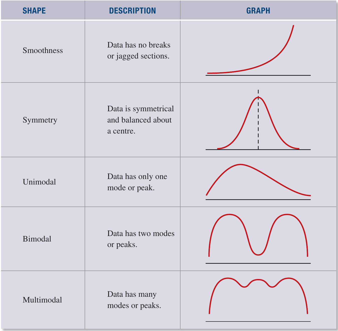
When working with data, we need to describe the overall shape and pattern of how values are distributed. The general shape of a distribution can be described using three main characteristics: smoothness, symmetry, and the number of modes.
A smooth distribution is one where data changes gradually without sudden breaks or irregular jumps. The pattern flows continuously from one value to the next.
Symmetry refers to whether the distribution is balanced evenly on both sides of a central vertical line. If you could fold the distribution along this centre line, both halves would match up like a mirror image.
The mode is the value that appears most frequently in the dataset (the peak with the highest frequency). Distributions can have different numbers of peaks or modes, which tells us about the pattern of the data.
Types of distribution shapes
Distributions can be classified based on how many peaks or modes they contain:
Unimodal distributions have a single peak or mode. Most of the data clusters around one central value, creating one high point in the distribution.
Bimodal distributions have two distinct peaks or modes. This often happens when you have two different groups mixed together in your dataset, each with its own typical value.
Multimodal distributions have many peaks or modes. This suggests the data comes from several different groups or sources, each contributing its own cluster of values.
Symmetry and skewness
Data is symmetric when it forms a mirror image of itself around a central vertical line. If you were to fold the distribution in half at the middle, both sides would match up perfectly. In symmetric distributions, the data is evenly balanced on both sides.
However, many real-world datasets are not symmetric. When data has more values concentrated on one side, we say it is skewed. The direction of the skew is determined by where the long tail of the distribution points.

Types of skewness
There are three main categories of skewness:
No skew (symmetric): The data is evenly balanced on both sides of a vertical centre line. The left and right halves are mirror images of each other.
Positively skewed: There is more data concentrated on the left side of the distribution, with a long tail extending toward the right (positive) side. The tail points in the positive direction along the number line. This often occurs with data like income or house prices, where most values are lower but a few are extremely high.
Negatively skewed: There is more data concentrated on the right side of the distribution, with a long tail extending toward the left (negative) side. The tail points in the negative direction along the number line. This might occur with test scores where most students score highly but a few score very low.
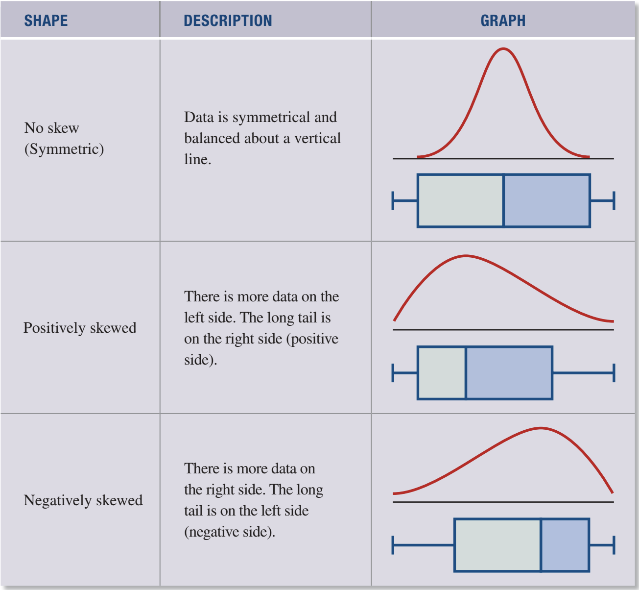
Remember that the skew is named after the direction of the tail, not where most of the data is located. Positive skew = tail to the right; negative skew = tail to the left.
Measures of location
Measures of location (also called measures of central tendency) tell us about the typical or central value in a dataset. The three main measures are the mean, median, and mode. Each has its own strengths and weaknesses, making them suitable for different situations.
Mean
The mean is calculated by adding up all the values and dividing by the number of values:
Advantages:
- Simple to understand and calculate
- Takes into account every single value in the dataset
- Most consistent across different samples from the same population
Disadvantages:
- Strongly influenced by extreme values (outliers)
- Cannot be used with categorical data (data in categories rather than numbers)
Median
The median is the middle value when all data values are arranged in order from smallest to largest.
Advantages:
- Simple to understand
- Not affected by outliers or extreme values
Disadvantages:
- May not represent the centre well in some distributions
- Data must be sorted before calculating
- Varies more than the mean when taking different samples from the same population
The median is particularly useful when your data contains outliers or is skewed, as it provides a more reliable measure of the centre than the mean in these cases.
Mode
The mode is the value that occurs most frequently in the dataset.
Advantages:
- Very simple to identify
- Not affected by outliers
- Can be used with categorical data (like favourite colours or types of pets)
Disadvantages:
- There may be no mode at all, or multiple modes
- May not represent the centre of the data well
Measures of spread
Measures of spread tell us how much the data values vary or are dispersed around the centre. The three main measures are the range, interquartile range, and standard deviation.
Range
The range is the difference between the highest and lowest values:
Advantages:
- Very simple to understand
- Quick and easy to calculate
Disadvantages:
- Only depends on the two extreme values (smallest and largest)
- Can be heavily distorted by a single outlier
Interquartile range (IQR)
The interquartile range is the difference between the upper quartile () and the lower quartile ():
This represents the spread of the middle 50% of the data.
Advantages:
- Straightforward to calculate for small datasets
- Easy to understand (focuses on middle 50% of data)
- Not affected by outliers
Disadvantages:
- More difficult to calculate for large datasets
- Only depends on the two quartile values
- Data must be sorted before calculating
The IQR is a robust measure of spread because it focuses on the central portion of the data, effectively ignoring the influence of extreme values on either end of the distribution.
Standard deviation
The standard deviation measures how far values typically deviate from the mean. It takes into account every value in the dataset.
Advantages:
- Uses every single data value
- Not significantly affected by outliers (compared to range)
Disadvantages:
- Complex to calculate without a calculator
- More difficult concept to understand
Comparison table
| Measure | Advantages | Disadvantages |
|---|---|---|
| Mean | - Easy to understand and calculate - Uses every score - Most consistent across samples | - Distorted by outliers - Not suitable for categorical data |
| Median | - Easy to understand - Not affected by outliers | - May not be central - Data needs sorting - Varies more than mean in samples |
| Mode | - Easy to determine - Not affected by outliers - Suitable for categorical data | - May be no mode or multiple modes - May not be central |
| Range | - Easy to understand - Easy to calculate | - Depends only on extreme values - Distorted by outliers |
| IQR | - Easy for small datasets - Easy to understand - Not affected by outliers | - Difficult for large datasets - Depends on quartiles only - Data needs sorting |
| Standard deviation | - Uses every score - Not significantly affected by outliers | - Difficult to calculate without calculator - Difficult to understand |
When choosing which measures to use, consider whether your data has outliers. If outliers are present, use median and IQR rather than mean and range. If the data is symmetric with no outliers, the mean and standard deviation are usually preferred.
Worked example: Comparing statistics for two sets of data
Worked Example: Analyzing Fitness Class Attendance
Let's look at a practical example comparing the number of participants in fitness classes for two instructors, Bec and Rita, across one week:
| Day | M | T | W | T | F | S | S |
|---|---|---|---|---|---|---|---|
| Bec | 8 | 5 | 4 | 8 | 8 | 4 | 5 |
| Rita | 10 | 9 | 12 | 14 | 8 | 10 | 1 |

Part a: Find the mean and median for each dataset
For Bec:
Calculate the mean:
To find the median, arrange the values in order:
Since there are 7 values (odd number), the median is the middle value (4th value):
Median
For Rita:
Calculate the mean:
Arrange the values in order:
The median is the middle value (4th value):
Median
Part b: Find the range and interquartile range for each dataset
For Bec:
Range
For IQR, we need the upper quartile () and lower quartile ():
IQR
For Rita:
Range
IQR
Part c: Examine the summary statistics and outline any concerns
Looking at Rita's data, there is a clear outlier: the value on Sunday. This extremely low value is separated from the rest of the data.
The presence of this outlier has significantly affected some of Rita's statistics:
- The mean has been pulled down (from what would be around 11 without the outlier to 9.1)
- The range has been greatly increased (from what would be about 6 to 13)
- The median and IQR remain more reliable as they are not affected by the single extreme value
This example shows why it's important to identify outliers and choose appropriate measures. For Rita's data, the median and IQR give a better representation of the typical class size than the mean and range.
Key Points to Remember:
- Distribution shapes can be described by smoothness (gradual changes), symmetry (balanced vs skewed), and number of modes (unimodal, bimodal, multimodal)
- Skewness is named after the tail direction: positive skew has a right tail, negative skew has a left tail
- Mean uses all values but is affected by outliers; median resists outliers but varies more between samples
- Range is simple but heavily influenced by extreme values; IQR focuses on the middle 50% and resists outliers
- When data contains outliers, prefer median and IQR over mean and range for more reliable summaries