Modelling Projectile Motion (HSC SSCE Physics): Revision Notes

Modelling Projectile Motion

Introduction to modelling in physics

Physicists use different types of models to understand physical systems, solve problems, and make predictions. When studying projectile motion, three main types of models are particularly useful: mathematical models, visual models, and numerical models.

Mathematical models

A mathematical model uses equations to describe the motion. For projectile motion, we treat it as a combination of two simpler types of motion happening simultaneously.

Projectile motion combines two rectilinear motions:

• Vertical motion: Uniformly accelerated motion due to gravity (acceleration = $g$)
• Horizontal motion: Constant velocity motion (zero acceleration)

The mathematical model uses:

• Constant acceleration kinematics equations for vertical motion
• Constant velocity equations for horizontal motion

This mathematical approach allows us to analyse and predict projectile behaviour precisely.

Visual or graphical models

Visual models provide graphical representations of projectile motion. These models help us see relationships clearly, such as how launch angle affects range. By plotting experimental data alongside the mathematical model, we can create visual representations that make patterns and relationships easier to understand.

Numerical models and computer simulations

A numerical model or computer simulation uses the mathematical equations to calculate the motion step by step over time. This type of model is particularly powerful because it can be easily modified to investigate different conditions, such as varying launch angle, initial velocity, or even gravity.

Investigation 2.3: Computer simulation of the trajectory of a projectile

Aim

To use spreadsheet software to model the trajectory of a projectile.

Materials

• Computer with spreadsheet software

Method

Initial setup:

Open a new file in your spreadsheet software and add a descriptive heading at the top. Save it with a suitable filename.

Step 1: Set up the initial conditions

The initial conditions define how the projectile starts its motion. These are:

• Initial velocity ($u$)
• Launch angle ($\theta$)
• Acceleration due to gravity ($g$)

In your spreadsheet, label cells above the values you enter. The setup should include:

• Cell B4: Launch angle in degrees (e.g., $30°$)
• Cell C4: Launch angle in radians using the command =RADIANS(B4)
• Cell D4: Acceleration due to gravity (e.g., $-9.8$ m/s²)

Calculate the components of initial velocity:

• Horizontal component: $u_x = u\cos\theta$
  • Cell A6: Use command =25*COS(C4) (where 25 is the initial velocity in m/s)
• Vertical component: $u_y = u\sin\theta$
  • Cell B6: Use command =25*SIN(C4)

Step 2: Calculate velocity as a function of time

Create three columns labelled: time ($t$), horizontal velocity ($v_x$), and vertical velocity ($v_y$).

Time column:

• First cell (A10): Enter $0$ (initial time)
• Next cell (A11): Enter command =A10+0.05 to increase time by 0.05 seconds
• Copy this command down the column (use Shift + Page Down to select many cells at once)

Horizontal velocity column ($v_x$):

• Cell B10 and all below: Enter command =$A$6

The horizontal velocity is constant throughout the motion and equals the initial horizontal velocity.

Vertical velocity column ($v_y$):

• Cell C10 and all below: Enter command =$B$6+A10*$D$4

This implements the equation $v_y = u_y + gt$, where the vertical velocity changes due to constant acceleration.

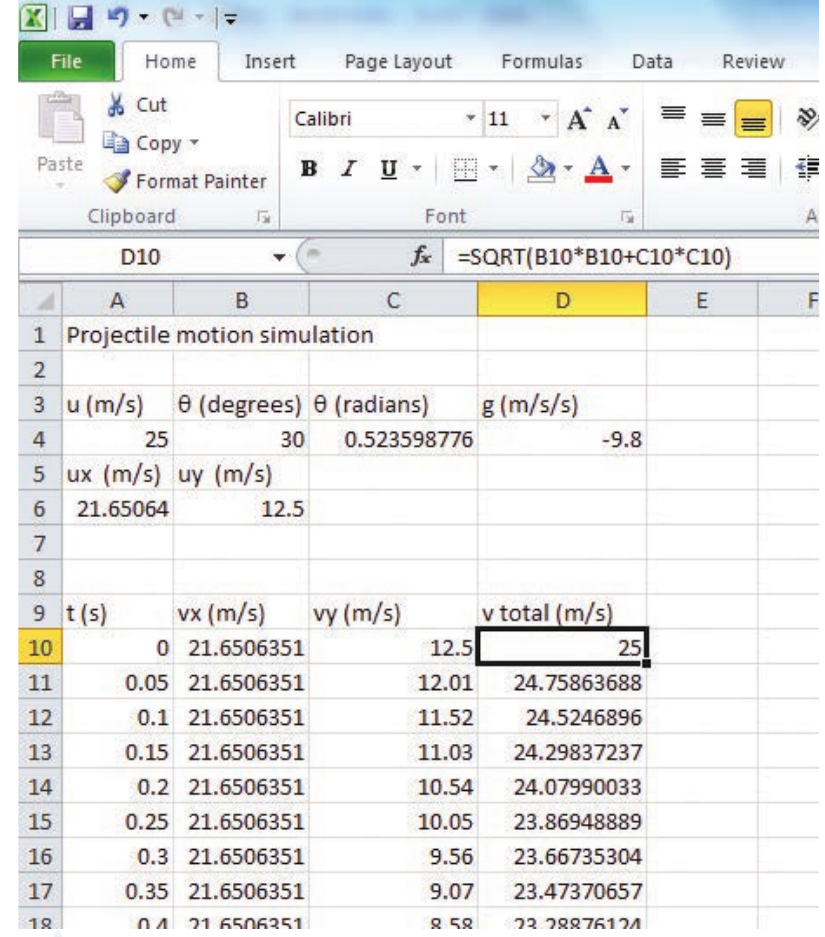
Total velocity column:

• Cell D10 and all below: Enter command =SQRT(B10B10+C10C10)

This calculates the magnitude of velocity using Pythagoras' theorem: $v_{\text{total}} = \sqrt{v_x^2 + v_y^2}$

Step 3: Calculate position as a function of time

Add two more columns labelled: horizontal position ($x$) and vertical position ($y$).

Horizontal position ($x$):

• Cell beneath the $x$ label: Enter command =$A$6*A10
• Copy to cells below

This implements $x = u_x t$ for constant velocity motion.

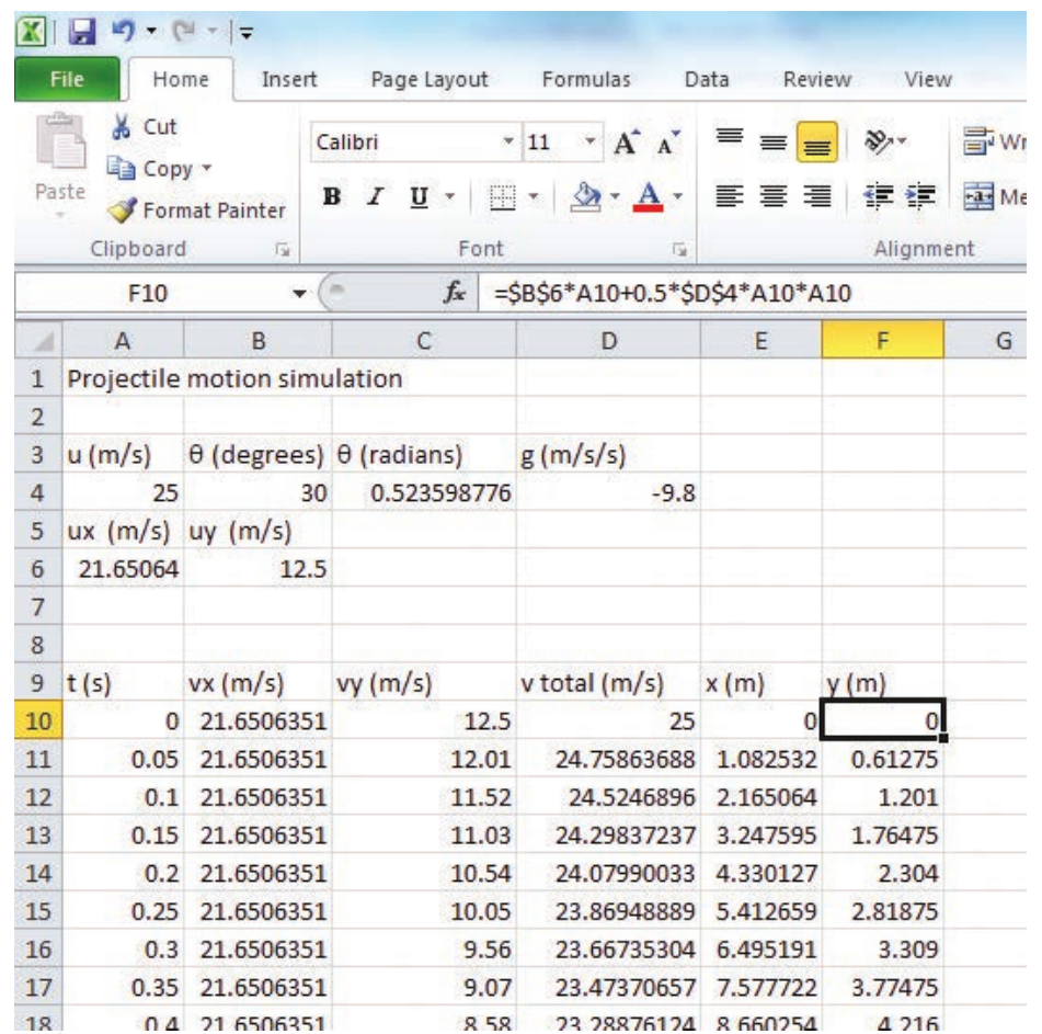
Vertical position ($y$):

• Cell beneath the $y$ label: Enter command =$B$6A10+0.5$D$4A10A10
• Copy to cells below

This implements $y = u_y t + \frac{1}{2}gt^2$ for uniformly accelerated motion.

Investigating different conditions:

To compare different conditions:

1. Copy your starting worksheet to create a duplicate
2. Modify the copy by changing one variable (e.g., launch angle)
3. Compare the results from both models

Results and analysis

Create the following scatter graphs:

1. Horizontal, vertical, and total velocity as functions of time
2. Horizontal, vertical, and total velocity as functions of position
3. Trajectory (vertical position as a function of horizontal position)

Discussion

Consider these questions when analysing your results:

1. Graph shapes: Comment on the shape of your graphs. Do they match what you expect based on:
   • Physical experiments with projectiles?
   • The equations used in the simulation?
2. Varying initial conditions: What happens when you change the initial conditions?
   • If you vary launch angle: What happens to range and maximum height?
   • If you vary $g$: What happens to time of flight, range, and maximum height?
3. Answer your inquiry question or state whether your hypothesis was supported.

Conclusion

Write a conclusion summarising the outcomes of your investigation. Include what you learned about projectile motion from creating and using the numerical model.

Benefits of computer simulations

Computer simulations offer several advantages:

• Easy to modify variables and test different scenarios
• Can visualise motion that might be difficult to observe experimentally
• Allows investigation of conditions that might be impractical in real experiments (e.g., different gravity values)
• Provides precise numerical data for analysis
• Helps develop understanding by connecting mathematical equations to visual representations