The Trajectory of a Charged Particle in a Uniform Electric Field Revision Notes for HSC SSCE Physics

The Trajectory of a Charged Particle in a Uniform Electric Field

Introduction to charged particle motion in electric fields

When a charged particle enters a uniform electric field, it experiences a constant force. The direction of this force depends on the sign of the charge:

Positive charges experience a force in the direction of the electric field
Negative charges experience a force opposite to the electric field direction

infoNote

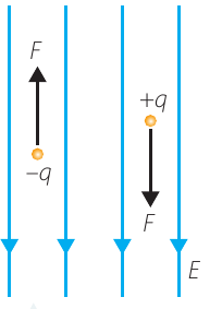
This behaviour differs significantly from gravitational fields, where all masses experience forces in the same direction. The charge sign determines whether the particle accelerates with or against the field - a key distinction that makes electric fields more versatile than gravitational fields for controlling particle motion.

Acceleration in a uniform electric field

Parallel to the field

A charged particle in a uniform electric field experiences constant acceleration parallel to the field direction. This acceleration is given by:

$a_{\parallel} = \frac{Eq}{m}$

where:

$E$ is the electric field strength (in $\text{V} \cdot \text{m}^{-1}$ )
$q$ is the charge of the particle (in $\text{C}$ )
$m$ is the mass of the particle (in $\text{kg}$ )

chatImportant

The sign of the charge determines the direction of acceleration: positive charges accelerate in the field direction, while negative charges accelerate opposite to the field. This is represented by the sign of $q$ in the equation.

Perpendicular to the field

When no other forces act on the particle, the acceleration perpendicular to the electric field is zero:

$a_{\perp} = 0$

This means the velocity component perpendicular to the field remains constant throughout the motion - a crucial insight for analyzing the trajectory.

Breaking motion into components

Consider a charged particle entering a uniform electric field with initial velocity $u$ at an angle $\theta$ to the field direction. We can break this initial velocity into two components:

Parallel to the field: $u_{\parallel} = u\cos\theta$

Perpendicular to the field: $u_{\perp} = u\sin\theta$

infoNote

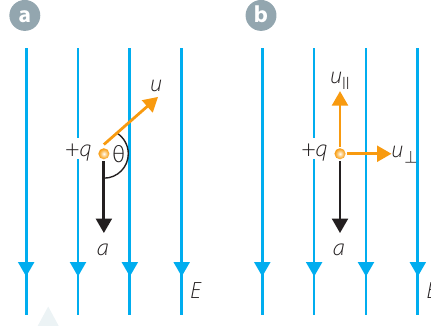
Important Convention: We measure the angle $\theta$ from the field direction, not from the horizontal. This convention is particularly useful because electric fields can point in any direction - they're not always vertical like gravitational fields.

Velocity equations

Using the kinematic equations for constant acceleration, we can find the velocity at any time $t$ . The motion separates neatly into two independent components:

Parallel to the field: $v_{\parallel} = u_{\parallel} + a_{\parallel}t = u_{\parallel} + \frac{Eq}{m}t$

Perpendicular to the field: $v_{\perp} = u_{\perp} + a_{\perp}t = u_{\perp}$

chatImportant

Remember: The perpendicular component stays constant because there is no acceleration in that direction. Only the parallel component changes with time. This is the key to understanding why the trajectory is parabolic.

Position equations

To find the position of the particle at any time, we apply the kinematic equations for constant acceleration. Starting from an initial position $(x_0, y_0)$ , and defining the field to point in the $y$ direction:

Parallel to the field (y-direction): $y = y_0 + u_{\parallel}t + \frac{1}{2}a_{\parallel}t^2 = y_0 + u_{\parallel}t + \frac{Eq}{2m}t^2$

Perpendicular to the field (x-direction): $x = x_0 + u_{\perp}t$

If we define the starting position as the origin (so $x_0 = 0$ and $y_0 = 0$ ):

$y = u_{\parallel}t + \frac{Eq}{2m}t^2$

$x = u_{\perp}t$

These equations reveal the mathematical structure of the motion: linear displacement perpendicular to the field combined with quadratic displacement parallel to the field produces the characteristic parabolic trajectory.

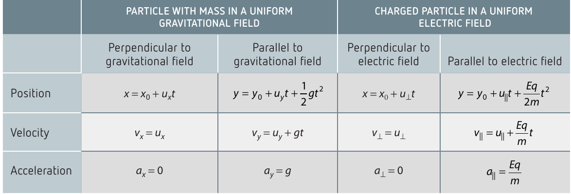
Comparison with projectile motion

The motion of a charged particle in a uniform electric field is mathematically identical to projectile motion in a uniform gravitational field. Both involve:

Constant velocity in one direction
Constant acceleration in a perpendicular direction
A parabolic trajectory

chatImportant

Key Analogy: The crucial insight is that gravitational acceleration $g$ is replaced by electric acceleration $\frac{Eq}{m}$ . All the projectile motion equations you learned can be applied here with this simple substitution!

However, there's a critical difference: In gravitational fields, all objects with mass accelerate downward (in the direction of $g$ ). In electric fields, the direction of acceleration depends on the charge sign - positive charges accelerate along the field, negative charges accelerate opposite to it.

The parabolic trajectory

A charged particle in a uniform electric field follows a parabolic path, just like a projectile near Earth's surface. The particle exhibits these characteristics:

Moves with constant velocity perpendicular to the field
Accelerates continuously parallel to the field
Combines these motions to produce a curved trajectory

infoNote

This motion can be modelled as a superposition of two simpler motions:

Rectilinear motion with constant velocity (perpendicular direction)
Rectilinear motion with constant acceleration (parallel direction)

Understanding this decomposition makes complex trajectories much easier to analyze!

Worked example: Dust particle between parallel plates

lightbulbExample

Worked Example: Motion of a Charged Dust Particle

Let's examine a practical calculation involving a charged dust particle entering an electric field between parallel plates.

Problem: A dust particle with mass $1.5 \times 10^{-5}$ kg and charge $-5.6 \times 10^{-9}$ C is falling vertically downward at $0.10$ m s $^{-1}$ when it enters the region between two vertical parallel charged plates. The electric field between the plates is $1500$ V m $^{-1}$ pointing to the right. Calculate:

a) The acceleration of the dust particle
b) The total velocity after 1.0 s
c) The displacement after 1.0 s

Assume all forces other than the electrostatic force are negligible.

Part a: Acceleration

Using the equation for acceleration in an electric field:

$a = \frac{Eq}{m}$

$a = \frac{(1500 \text{ V} \cdot \text{m}^{-1})(-5.6 \times 10^{-9} \text{ C})}{1.5 \times 10^{-5} \text{ kg}}$

$a = -0.56 \text{ m} \cdot \text{s}^{-2}$

The acceleration is 0.56 m s $^{-2}$ pointing to the left (the negative sign indicates direction opposite to the field).

Part b: Velocity after 1.0 s

The motion has two components:

Perpendicular to the field (vertical): $v_{\perp} = u_{\perp} = 0.10 \text{ m} \cdot \text{s}^{-1} \text{ downward}$

Parallel to the field (horizontal): $v_{\parallel} = u_{\parallel} + \frac{Eq}{m}t = 0 + \frac{(1500)(-5.6 \times 10^{-9})}{1.5 \times 10^{-5}}(1.0)$

$v_{\parallel} = -0.56 \text{ m} \cdot \text{s}^{-1} \text{ (to the left)}$

Total velocity magnitude: $v = \sqrt{v_{\parallel}^2 + v_{\perp}^2} = \sqrt{(-0.56)^2 + (-0.10)^2}$

$v = 0.57 \text{ m} \cdot \text{s}^{-1}$

Part c: Displacement after 1.0 s

Vertical displacement (perpendicular to field): $y = y_0 + u_{\perp}t = 0 + (-0.10)(1.0) = -0.10 \text{ m}$

The particle moves 0.10 m downward.

Horizontal displacement (parallel to field): $x = x_0 + u_{\parallel}t + \frac{Eq}{2m}t^2$

$x = 0 + 0 + \frac{(1500)(-5.6 \times 10^{-9})}{2(1.5 \times 10^{-5})}(1.0)^2 = -0.28 \text{ m}$

The particle moves 0.28 m to the left.

Final Result: After 1.0 second, the particle has moved 0.28 m left and 0.10 m down from its entry point, following a parabolic path.

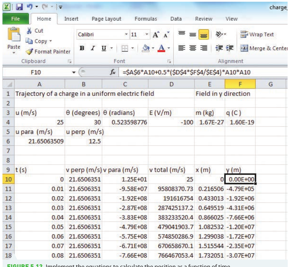
Investigation: Computer simulation of trajectory

You can model the trajectory of a charged particle using spreadsheet software. This allows you to investigate how changing the charge, mass, field strength, or initial velocity affects the motion - a powerful tool for developing intuition about electric field dynamics.

Setting up the simulation

infoNote

Step 1: Define initial conditions

Create cells for the fundamental parameters:

Initial velocity $u$ (in m s $^{-1}$ )
Angle $\theta$ to the field (in degrees and radians)
Electric field strength $E$ (in V m $^{-1}$ )
Particle mass $m$ (in kg)
Particle charge $q$ (in C)

Then calculate the initial velocity components:

Parallel component: $u_{\parallel} = u\cos\theta$
Perpendicular component: $u_{\perp} = u\sin\theta$

infoNote

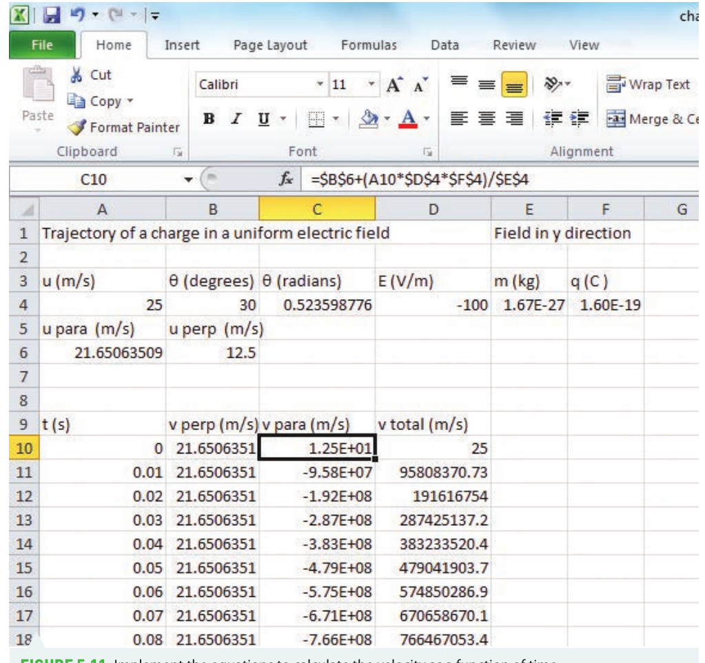
Step 2: Calculate velocity as a function of time

Create columns for time-dependent quantities:

Time $t$ (incremented by small steps, e.g., 0.01 s)
Perpendicular velocity: $v_{\perp} = u_{\perp}$ (constant throughout)
Parallel velocity: $v_{\parallel} = u_{\parallel} + \frac{Eq}{m}t$
Total velocity magnitude: $v = \sqrt{v_{\parallel}^2 + v_{\perp}^2}$

This allows you to track how the velocity vector changes over time.

infoNote

Step 3: Calculate position as a function of time

Add columns for spatial coordinates:

x-position: $x = u_{\perp}t$
y-position: $y = u_{\parallel}t + \frac{Eq}{2m}t^2$

These equations will generate the parabolic trajectory when plotted.

Exploring the simulation

Once your spreadsheet is set up, you can investigate how different variables affect the trajectory:

Change the charge: Model electrons (negative charge), protons (positive charge), or alpha particles (double positive charge)
Change the mass: Compare light particles like electrons with heavy particles like alpha particles
Change the field: Model fair-weather conditions ( $E = 100$ V m $^{-1}$ ) or stormy weather conditions
Change initial velocity: Vary the speed and angle of entry to see how trajectory shape changes

Analysis

Create graphs to visualize the motion and verify your understanding:

Velocity vs time graph: Should show how the parallel velocity changes linearly while perpendicular velocity remains constant
Trajectory graph: Plot y-position vs x-position to see the characteristic parabolic path

chatImportant

The graphs should confirm that charged particles follow parabolic trajectories, similar to projectiles in gravitational fields. Any deviations suggest errors in your setup or calculations.

Key exam tips

bookmarkSummary

Essential Exam Strategy:

Always identify whether the particle is positive or negative - this determines the direction of acceleration
Break the motion into parallel and perpendicular components immediately - this simplifies the problem dramatically
Remember: perpendicular velocity is constant, parallel velocity changes linearly
Check units carefully in calculations, especially for charge (C) and field strength (V m $^{-1}$ )
The trajectory equations are identical to projectile motion, but replace $g$ with $\frac{Eq}{m}$
Draw a clear diagram showing the field direction, initial velocity, and acceleration before starting calculations

Summary

bookmarkSummary

Key Points to Remember:

A charged particle in a uniform electric field experiences constant acceleration parallel to the field and zero acceleration perpendicular to it
The trajectory is parabolic, identical in form to projectile motion in a gravitational field
Positive charges accelerate in the direction of the electric field; negative charges accelerate opposite to the field direction
Key equation for acceleration: $a_{\parallel} = \frac{Eq}{m}$
The motion can be analyzed by breaking it into perpendicular (constant velocity) and parallel (constant acceleration) components
All projectile motion techniques apply - just substitute $\frac{Eq}{m}$ for $g$

The Trajectory of a Charged Particle in a Uniform Electric Field (HSC SSCE Physics): Revision Notes