Constant Rate of Change Revision Notes for VCE SSCE Mathematical Methods

Constant Rate of Change

What is constant rate of change?

When we talk about a constant rate of change, we mean that something is changing at the same rate throughout. Think of driving a car at a steady speed - you're covering the same distance every minute. This steady, unchanging pattern is what we call a constant rate of change.

Linear functions are special because they always have a constant rate of change. If you have a function in the form $f(x) = mx + c$ , the rate of change is simply $m$ - the gradient of the line. This gradient stays the same no matter where you look on the graph.

infoNote

For any linear function, the rate of change equals the gradient of its graph. This is a fundamental property that makes linear functions predictable and easy to work with.

Finding the constant rate

There are two main ways to find the constant rate of change:

From the graph: Calculate the gradient by finding the change in the vertical direction divided by the change in the horizontal direction. The gradient of a straight line is the same between any two points you choose.

From the function rule: If the function is written as $f(x) = mx + c$ , then m is the constant rate of change. For example, if $f(x) = 3x + 2$ , the constant rate of change is 3.

chatImportant

Two methods to find constant rate:

Graphically: Calculate gradient = $\frac{\text{vertical change}}{\text{horizontal change}}$
Algebraically: Identify the coefficient $m$ in the function $f(x) = mx + c$

Both methods will give you the same result for a linear function!

Worked example: calculating speed from a distance-time graph

A car travels from Copahunga to Charlegum, which is a distance of $150$ km, in $2$ hours ( $120$ minutes). Assuming the car travels at a constant speed, we can draw a distance-time graph and calculate the speed.

lightbulbExample

Worked Example: Finding Speed from a Distance-Time Graph

Setting up the problem:

Let's call the distance function $D$ , where $D(t)$ represents the distance traveled after $t$ minutes.

Since the car travels at constant speed, the graph will be a straight line starting from the origin.

After $120$ minutes, the car has traveled $150$ km, so the point $(120, 150)$ is on our graph.

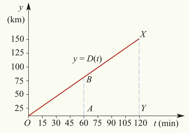
Finding the function rule:

The gradient of the line is:

\text{gradient} = \frac{\text{change in distance}}{\text{change in time}} = \frac{150}{120} = \frac{5}{4}

Since the line passes through the origin, the function is:

D(t) = \frac{5}{4}t

Interpreting the gradient:

The gradient of the graph gives us the speed. Therefore, the speed of the car is $\frac{5}{4}$ kilometres per minute.

Converting units:

To express this in kilometres per hour, we multiply by $60$ (since there are $60$ minutes in an hour):

\text{Speed} = \frac{5}{4} \times 60 = 75 \text{ km/h}

Therefore, the car is traveling at 75 km/h.

Worked example: comparing different constant rates

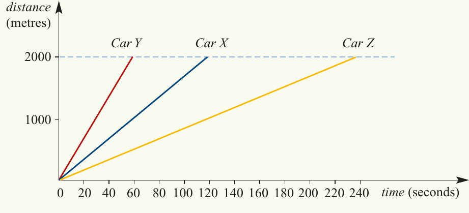
Three cars are driven over a $2$ -kilometre straight track from point A to point B. Each car travels at constant speed, but:

Car Y travels at twice the speed of car X
Car Z travels at half the speed of car X
Car X travels at $1$ km/min

We can illustrate this situation with a distance-time graph.

lightbulbExample

Worked Example: Comparing Multiple Constant Rates

Understanding the graph:

Each car's journey is represented by a straight line starting from the origin. The steeper the line, the faster the car is traveling.

Calculating the gradients:

For car X:

\text{gradient} = \frac{2000}{120} = 16\frac{2}{3} \text{ metres per second}

For car Y:

\text{gradient} = \frac{2000}{60} = 33\frac{1}{3} \text{ metres per second}

For car Z:

\text{gradient} = \frac{2000}{240} = 8\frac{1}{3} \text{ metres per second}

Key observation: Car Y has the steepest gradient and reaches the $2000$ metre mark first. Car Z has the gentlest gradient and takes the longest time. The gradient of each line directly represents the speed of that car.

infoNote

When an object's motion can be described by a linear distance-time graph, the object is traveling at a constant speed. This constant speed equals the gradient of the line.

Real-world applications of constant rate

Distance-time graphs are just one example of how constant rates appear in real life. Any situation that can be modeled with a straight-line graph involves a constant rate of change.

Currency exchange

Currency exchange is another perfect example. When you exchange money between two currencies, the exchange rate is constant (at any given time).

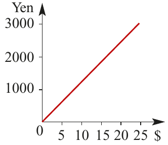
The graph shows the conversion between dollars and yen. The gradient of this straight line gives us the exchange rate - how many yen you get for each dollar.

infoNote

Understanding the gradient: If the line passes through the point $(20, 2400)$ , the gradient is $\frac{2400}{20} = 120$ . This means the exchange rate is 120 yen per dollar.

The gradient directly tells you the conversion rate between the two currencies!

Other examples

Many other situations involve constant rates:

Water filling a container at steady rate: Volume increases linearly with time
Constant pay rate: Earnings increase linearly with hours worked
Unit pricing: Total cost increases linearly with quantity purchased

In all these situations, the gradient of the straight-line graph represents the rate at which one quantity changes with respect to another.

bookmarkSummary

Key Points to Remember:

Linear functions have a constant rate of change equal to their gradient
For $f(x) = mx + c$ , the constant rate of change is m
In distance-time graphs, the gradient represents speed when traveling at constant velocity
Steeper gradients mean faster rates of change
Many real-world situations (like currency exchange and constant speed motion) can be modeled with linear functions
The rate of change can be calculated from the graph or read directly from the function rule

Constant Rate of Change (VCE SSCE Mathematical Methods): Revision Notes