Position and Average Velocity Revision Notes for VCE SSCE Mathematical Methods

Position and Average Velocity

Understanding how objects move in a straight line is a key application of rates of change. This topic introduces the fundamental concepts of position and velocity for particles moving along a line.

Position

Position tells us where a particle is located relative to a chosen reference point.

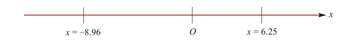
When studying motion along a straight line, we select a reference point called $O$ . This point acts as our zero position marker. We then adopt a sign convention to describe locations on either side of this reference point.

chatImportant

Sign convention:

Positions to the right of $O$ are positive
Positions to the left of $O$ are negative

For example, if a particle has position $x = 6.25$ metres, it is located $6.25$ metres to the right of $O$ . If its position is $x = -8.96$ metres, it is $8.96$ metres to the left of $O$ .

Position-time graphs

We can represent a particle's motion using a position-time graph, where time $t$ is shown on the horizontal axis and position $x$ is shown on the vertical axis.

Consider a particle that starts from rest at the origin and moves to the right. At $t = 5$ seconds, it stops and reverses direction. Here's what the motion looks like:

At time $t = 0$ : position $x = 0$ (particle at origin $O$ )
At time $t = 5$ : position $x = 6.25$ (particle has moved right)
At time $t = 8$ : position $x = -8.96$ (particle has moved left past $O$ )

infoNote

From the graph, we can observe:

For $0 < t < 7.1$ , the position is positive, so the particle is to the right of $O$
For $t > 7.1$ , the position is negative, so the particle is to the left of $O$

Average velocity

Average velocity measures how quickly a particle's position changes over a time interval. It is the average rate of change in position with respect to time.

Formula:

\text{average velocity} = \frac{\text{change in position}}{\text{change in time}}

The units for average velocity are typically metres per second (m/s) when position is measured in metres and time in seconds.

Calculating average velocity

Using the particle motion described earlier, we can calculate average velocity for different time intervals.

For the interval $0 \leq t \leq 5$ :

Change in position: $6.25 - 0 = 6.25$ metres

Change in time: $5 - 0 = 5$ seconds

\text{average velocity} = \frac{6.25}{5} = 1.25 \text{ m/s}

For the interval $5 \leq t \leq 8$ :

Change in position: $-8.96 - 6.25 = -15.21$ metres

Change in time: $8 - 5 = 3$ seconds

\text{average velocity} = \frac{-15.21}{3} = -5.07 \text{ m/s}

infoNote

Notice that the average velocity is negative in the second interval. This indicates that the particle is moving in the negative direction (to the left).

Worked example

lightbulbExample

Worked Example: Finding Average Velocity

A particle moves in a straight line with position function $s(t) = 6t - t^2$ , where $t$ is measured in seconds and $s$ is measured in metres.

Part a: Find the average velocity for the time interval $[0, 1]$ .

First, find the position at each time:

s(0) = 6(0) - 0^2 = 0

s(1) = 6(1) - 1^2 = 5

Calculate the average velocity:

\text{average velocity} = \frac{\text{change in position}}{\text{change in time}}

The average velocity for $[0, 1]$ is 5 m/s.

Part b: Find the average velocity for the time interval $[6, 8]$ .

Find the position at each time:

s(6) = 6(6) - 6^2 = 36 - 36 = 0

s(8) = 6(8) - 8^2 = 48 - 64 = -16

Calculate the average velocity:

\text{average velocity} = \frac{\text{change in position}}{\text{change in time}}

The average velocity for $[6, 8]$ is -8 m/s.

Velocity-time graphs

When the position-time graph consists of straight line segments (representing constant velocity during each segment), we can construct a corresponding velocity-time graph. The velocity during each segment equals the gradient of that segment on the position-time graph.

Worked example: bicycle trip

lightbulbExample

Worked Example: Bicycle Trip

A boy lives on a long straight road running north-south. He chooses north as the positive direction. The graph below shows his position over time during a bicycle trip.

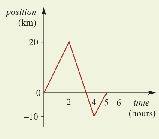
Part a: Describe the trip.

First segment (0 to 2 hours):

The boy travels north for $2$ hours.

His velocity is:

\frac{20 - 0}{2} = 10 \text{ km/h}

Second segment (2 to 4 hours):

He turns and rides south for $2$ hours.

His velocity is:

\frac{-10 - 20}{2} = \frac{-30}{2} = -15 \text{ km/h}

Third segment (4 to 5 hours):

He turns and rides north until reaching home.

His velocity is:

\frac{0 - (-10)}{1} = 10 \text{ km/h}

Part b: Draw the velocity-time graph.

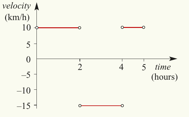
The velocity-time graph shows three horizontal segments corresponding to the three periods of constant velocity.

Worked example: particle with constant velocity segments

lightbulbExample

Worked Example: Particle Motion with Constant Velocity

A particle starts at rest at point $O$ and moves to the right with constant velocity, reaching point $A$ ( $15$ metres from $O$ ) after $5$ seconds. It then returns to $O$ , taking $10$ seconds for the return trip.

We can draw both the position-time and velocity-time graphs on one set of axes.

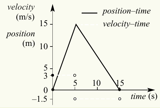
Explanation:

The gradient of the position-time graph for $0 < t < 5$ is:

\frac{15 - 0}{5 - 0} = 3 \text{ m/s}

The gradient for $5 < t < 15$ is:

\frac{0 - 15}{15 - 5} = -1.5 \text{ m/s}

The gradient of the position-time graph determines the velocity at each moment, which gives us the velocity-time graph.

Instantaneous velocity

While average velocity tells us the overall rate of change over an interval, instantaneous velocity tells us the rate of change at a specific moment in time.

chatImportant

Instantaneous velocity is the instantaneous rate of change in position with respect to time. Graphically, it equals the gradient of the tangent to the position-time graph at a particular point.

If we know the instantaneous velocity at every moment, we can sketch a velocity-time graph even when the particle doesn't move with constant velocity.

Relationship between position and velocity

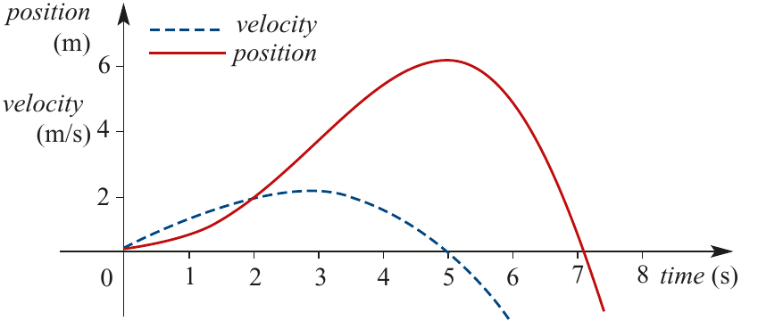
This graph shows both position and velocity for the same particle motion. The vertical axis represents both metres per second (for velocity) and metres (for position).

Key observations:

For $0 < t < 5$ : velocity is positive, so the particle travels from left to right
For $t > 5$ : velocity is negative, so the particle travels from right to left
At $t = 5$ : velocity is zero, so the particle is instantaneously at rest

infoNote

Notice that the velocity graph shows the gradient of the position graph at each moment. Where the position graph has a positive gradient, the velocity is positive. Where the position graph has a negative gradient, the velocity is negative.

Worked example: estimating instantaneous velocity

lightbulbExample

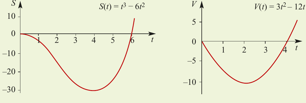
Worked Example: Estimating Instantaneous Velocity

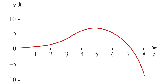
The position of a particle is given by $S(t) = t^3 - 6t^2$ for $t \geq 0$ . The velocity function is $V(t) = 3t^2 - 12t$ .

Part a: Find the average velocity for the intervals:

i) $[3.5, 4.5]$ :

\text{Average velocity} = \frac{S(4.5) - S(3.5)}{4.5 - 3.5}

ii) $[3.9, 4.1]$ :

\text{Average velocity} = \frac{S(4.1) - S(3.9)}{4.1 - 3.9}

iii) $[3.99, 4.01]$ :

\text{Average velocity} = \frac{S(4.01) - S(3.99)}{4.01 - 3.99}

Part b: What is the instantaneous velocity when $t = 4$ ?

The results from part a show that as the interval gets smaller around $t = 4$ , the average velocity approaches zero. This suggests the instantaneous velocity at $t = 4$ is 0 m/s, which is confirmed by both graphs.

Part c: When is the velocity positive or negative?

i) From the position-time graph, velocity is positive for $t > 4$ (when the gradient is positive).

ii) From the position-time graph, velocity is negative for $0 < t < 4$ (when the gradient is negative).

Remember!

bookmarkSummary

Key Points to Remember:

Position specifies a particle's location relative to a reference point $O$ , with positive positions to the right and negative positions to the left
Average velocity is calculated as $\displaystyle\frac{\text{change in position}}{\text{change in time}}$ and represents the overall rate of change over an interval
Instantaneous velocity is the rate of change at a specific moment and equals the gradient of the tangent to the position-time graph
The gradient of a position-time graph gives the velocity at that point
When velocity is positive, the particle moves in the positive direction; when negative, it moves in the negative direction
When velocity equals zero, the particle is instantaneously at rest

Position and Average Velocity (VCE SSCE Mathematical Methods): Revision Notes