Approximating the Distribution of the Sample Proportion Revision Notes for VCE SSCE Mathematical Methods

Approximating the Distribution of the Sample Proportion

Introduction

When working with sample proportions, we often need to calculate probabilities for different sample outcomes. While we can determine the exact distribution of a sample proportion using probability theory, this approach is only practical for small sample sizes (typically less than 10). In real-world situations, we usually work with much larger samples, which makes exact calculations impractical. Fortunately, we can overcome this limitation by using an approximation method based on the normal distribution.

infoNote

For samples with fewer than 10 observations, we can calculate exact probabilities using the binomial distribution. However, as sample sizes increase, these calculations become increasingly complex and time-consuming, making the normal approximation both practical and necessary.

Understanding sample proportion variation

Let's explore this concept with a practical example. Suppose we know that 55% of people in Australia have blue eyes, so the population proportion is $p = 0.55$ . We're interested in understanding what values of the sample proportion $\hat{p}$ we might observe when we take random samples of size 100 from this population.

Single sample observations

If we select one sample of 100 people and find that 50 have blue eyes, the sample proportion is:

\hat{p} = \frac{50}{100} = 0.5

If we select a second sample of 100 people and this time 58 have blue eyes, the sample proportion for this second sample is:

\hat{p} = \frac{58}{100} = 0.58

infoNote

Notice that even though both samples come from the same population, they yield different sample proportions. This variation is a natural consequence of random sampling.

Visualising multiple samples

When we continue this sampling process and take 10 samples, the observed values of $\hat{p}$ might look like this:

From this dotplot, we can see that the proportion of people with blue eyes varies from sample to sample. In these particular 10 samples, the sample proportion ranges from as low as 0.44 to as high as 0.61.

The pattern emerges with more samples

What happens when we increase the number of samples? The following dotplot shows the distribution of sample proportions when 200 samples (each of size 100) were selected:

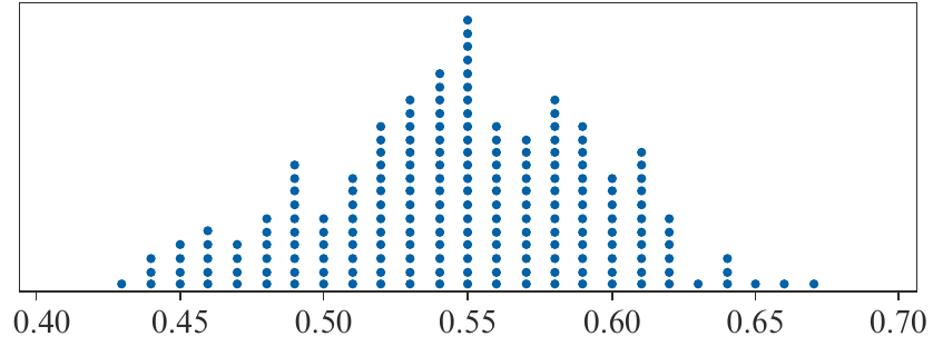
We can observe several important features:

The distribution is reasonably symmetric
The values are centred around 0.55 (the population proportion)
The values range from approximately 0.43 to 0.67

When we repeat this experiment with another 200 samples from the same population, we get:

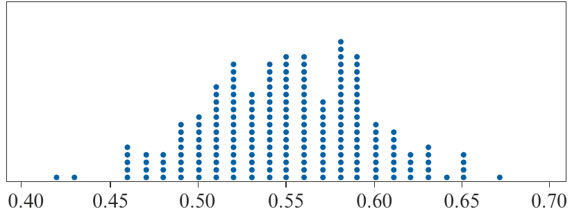
Again, the distribution is:

Reasonably symmetric
Centred at 0.55
Ranging from approximately 0.42 to 0.67

chatImportant

Key Principle: While there will be variation in the specific details each time we collect samples, the distribution of sample proportions tends to follow a predictable pattern in terms of shape, centre, and spread. This predictability is what allows us to use the normal approximation effectively.

The normal approximation

The predictable pattern we observe has a theoretical foundation. We know from probability theory that when the sample size is large enough, the distribution of a binomial random variable can be well approximated by a normal distribution.

Rule of thumb for approximation

chatImportant

Normal Approximation Conditions

The normal approximation to the binomial distribution is appropriate when:

Both $np > 5$ and $n(1-p) > 5$

The sample proportion $\hat{P}$ can be considered a linear function of a binomial random variable, which means the normal approximation also applies to the distribution of sample proportions.

The approximation formula

infoNote

Normal Approximation for Sample Proportions

When the sample size $n$ is large, the sample proportion $\hat{P}$ has an approximately normal distribution with:

Mean: $\mu = p$

Standard deviation:

\sigma = \sqrt{\frac{p(1-p)}{n}}

For our blue eyes example with $n = 100$ and $p = 0.55$ :

\mu = E(\hat{P}) = 0.55

\sigma = \text{sd}(\hat{P}) = \sqrt{\frac{0.55 \times 0.45}{100}} = 0.0497

Investigating with technology

We can use a calculator to simulate the sampling process and verify the normal approximation.

lightbulbExample

Worked Example: Using Technology to Simulate Sampling

Question: Assume that 55% of people in Australia have blue eyes. Use your calculator to illustrate a possible distribution of sample proportions $\hat{p}$ that may be obtained when 200 different samples (each of size 100) are selected from the population.

Solution using TI-Nspire:

Step 1: Generate the sample proportions

Start from a Lists & Spreadsheet page
Name the list propblue in Column A
In the formula cell of Column A, enter the formula: = randbin(100, 0.55, 200)/100

Table

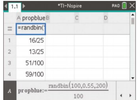
The syntax for this function is: randbin(sample size, population proportion, number of samples). We divide by the sample size to convert counts to proportions.

Step 2: Display the distribution

Insert a Data & Statistics page
Click on 'Click to add variable' on the horizontal axis and select propblue
A dotplot is displayed

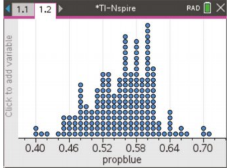
You can recalculate the random sample proportions using ctrl+R while in the Lists & Spreadsheet page.

Step 3: Fit a normal curve to the distribution

Menu > Plot Type > Histogram
Menu > Analyze > Show Normal PDF

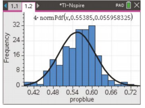
The calculated normal PDF is superimposed on the plot, showing the mean and standard deviation of the sample proportion.

Step 4: Obtain statistics from the distribution

Navigate to Calc > One-Variable
The results show that the mean of the sample proportions estimates the population proportion

Using the normal approximation

lightbulbExample

Worked Example: Finding Probabilities

Question: Assume that 60% of people have a driver's licence. Using the normal approximation, find the approximate probability that, in a randomly selected sample of size 200, more than 65% of people have a driver's licence.

Solution:

Step 1: Identify the given information

Given: $n = 200$ and $p = 0.6$

Step 2: Determine the distribution parameters

Since $n$ is large, the distribution of $\hat{P}$ is approximately normal with:

\mu = p = 0.6

\sigma = \sqrt{\frac{0.6(1-0.6)}{200}} = \sqrt{\frac{0.6 \times 0.4}{200}} = 0.0346

Step 3: Calculate the required probability

We need to find $\text{Pr}(\hat{P} > 0.65)$ .

Using the normal distribution with mean 0.6 and standard deviation 0.0346:

\text{Pr}(\hat{P} > 0.65) = 0.0745 \text{ (correct to four decimal places)}

lightbulbExample

Worked Example: Finding Sample Size

Question: Suppose again that 60% of people have a driver's licence, and that a random sample of size $n$ is selected from the population. If the probability that the proportion of people in the sample with a driver's licence is less than 58% is equal to 0.3446, what size sample was chosen?

Solution:

Step 1: Identify the given information

Given: $p = 0.6$ and $\text{Pr}(\hat{P} < 0.58) = 0.3446$ , find $n$ .

We assume $n$ is large enough for the normal approximation to apply.

Step 2: Set up the distribution parameters

The distribution of $\hat{P}$ is approximately normal with:

\mu = E(\hat{P}) = 0.60

\sigma = \text{sd}(\hat{P}) = \sqrt{\frac{0.6 \times 0.4}{n}} = \sqrt{\frac{0.24}{n}}

Step 3: Standardize and use the inverse normal

Converting to the standard normal distribution:

\text{Pr}(\hat{P} < 0.58) = \text{Pr}\left(Z < \frac{-0.02}{\sqrt{0.24/n}}\right) = 0.3446

Using the inverse normal function with probability 0.3446:

\frac{-0.02}{\sqrt{0.24/n}} \approx -0.400

Step 4: Solve for $n$

-0.02 = -0.400 \times \sqrt{\frac{0.24}{n}}

0.02 = 0.400 \times \sqrt{\frac{0.24}{n}}

0.05 = \sqrt{\frac{0.24}{n}}

0.0025 = \frac{0.24}{n}

n = \frac{0.24}{0.0025} = 96

Therefore, the sample size was 96.

bookmarkSummary

Key Points to Remember:

For small samples (less than 10), use the exact binomial distribution to find probabilities for sample proportions
For large samples, the normal approximation is more practical and efficient
The sample proportion $\hat{P}$ has an approximately normal distribution when $n$ is large, with mean $\mu = p$ and standard deviation $\sigma = \sqrt{\frac{p(1-p)}{n}}$
The rule of thumb for using the normal approximation is that both $np > 5$ and $n(1-p) > 5$
The mean of the sample proportions from repeated samples estimates the population proportion
Technology can be used to simulate sampling distributions and verify the normal approximation

Approximating the Distribution of the Sample Proportion (VCE SSCE Mathematical Methods): Revision Notes