Modelling Radioactive Decay (VCE SSCE Physics): Revision Notes
Modelling Radioactive Decay
Introduction to radiocarbon dating
Radiocarbon dating is a powerful scientific technique that allows us to determine the age of objects containing organic material. This method relies on measuring the decay of radioactive carbon-14 atoms present in the sample.
A remarkable example of radiocarbon dating in action comes from the Warratyi rock shelter in the Flinders Ranges, South Australia. Scientists from the Australian Nuclear Science and Technology Organisation (ANSTO) used radiocarbon dating to discover that Aboriginal peoples settled in this arid region approximately 49,000 years ago. This technique is reliable for dating objects up to 55,000-60,000 years old.
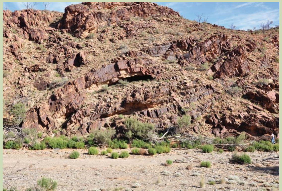
The Warratyi site provided evidence of extinct Australian megafauna, the earliest-known use of ochre in Australia and Southeast Asia, and early bone tools. This shows how radioactive decay can unlock secrets of human history.
Understanding random decay
The random nature of radioactive decay
Radioactive decay occurs as a completely random process. This means it is impossible to predict exactly when any particular radioactive nucleus will decay, regardless of how long the atom has existed. Think of it like this: you cannot tell which specific atom will decay next, just as you cannot predict which specific person in a crowd will sneeze next.
However, when dealing with large numbers of nuclei, we can make statistical predictions about the behaviour of the entire group. For example, one gram of uranium-238 contains approximately radioactive atoms. With such enormous numbers, we can accurately predict the overall decay rate using the concept of half-life.
Key Insight: Individual decay events are random and unpredictable, but the behaviour of large groups of radioactive nuclei follows predictable statistical patterns. This is why we can reliably use radioactive decay for dating and other applications.
Simulating decay with dice
A practical way to understand random decay is through a dice simulation. Here's how it works:
- Start with 120 dice
- Roll all the dice
- Remove all dice showing a particular number (say, 6)
- Count the remaining dice
- Repeat the process
This models radioactive decay because:
- You cannot predict which individual dice will show a 6 (randomness)
- Approximately one-sixth of all dice will show a 6 each time (statistical prediction)
- The number of "active" dice decreases with each roll (decay over time)
Dice Simulation Data
Here's an example of data from such an experiment:
| Roll | 0 | 1 | 2 | 3 | 4 | 5 | 6 | 7 | 8 | 9 |
|---|---|---|---|---|---|---|---|---|---|---|
| Dice remaining | 120 | 101 | 84 | 71 | 59 | 50 | 42 | 36 | 30 | 25 |
Notice that after approximately four rolls, about half the original dice remain. If each roll takes 5 minutes, the half-life for removing dice showing a 6 is approximately 20 minutes. If we changed the rule to remove all odd-numbered dice instead, the half-life would be much shorter - close to one roll or 5 minutes.
Half-life concept
Definition of half-life
Half-life is the time taken for half of a group of unstable nuclei to decay. It serves as a measure of the decay rate for any radioactive isotope.
For example, technetium-99m (a medical radioisotope) has a half-life of 6.0 hours. This means that after 6.0 hours, exactly half of the original technetium-99m nuclei will have decayed. After another 6.0 hours (total of 12.0 hours), only one-quarter of the original mass remains.
Range of half-lives
Different radioisotopes decay at vastly different rates:
- Very short half-lives: Francium-218 has millisecond
- Very long half-lives: Uranium-238 has million years
Natural and artificial radioisotopes
Radioisotopes can be classified as either natural (occurring in nature) or artificial (human-made). Here's a comparison:
| Isotope | Emission | Half-life | Application |
|---|---|---|---|
| Natural | |||
| Lead-210 | β⁻ | 22.2 years | Lead dating of sand and soil |
| Radium-88 | α | 1600 years | Historical medical uses |
| Carbon-14 | β⁻ | 5730 years | Carbon dating |
| Uranium-238 | α | 4500 million years | Nuclear fuel, geological dating |
| Artificial | |||
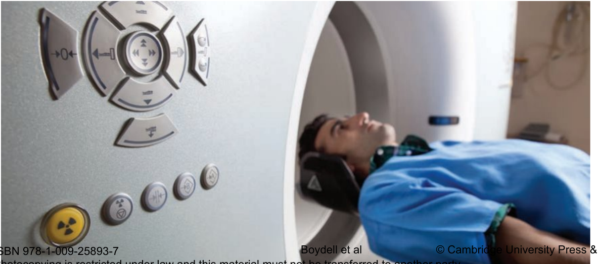
| Fluorine-18 | β⁺ | 110 minutes | PET scans |
| Technetium-99m | β⁻ | 6.0 hours | Medical tracer |
| Iodine-131 | β⁻ | 8 days | Medical tracer, radiation therapy |
| Iodine-125 | γ | 60 days | Internal radiation therapy |
| Cobalt-60 | γ | 5.3 years | External radiation therapy |
| Americium-241 | α | 460 years | Smoke detectors |
| Plutonium-239 | α | 24,100 years | Nuclear reactor fuel |
Properties of half-life
Critical Properties of Half-life
The half-life of any radioactive isotope is:
- Constant - it never changes for that isotope
- Unaffected by external conditions - temperature, magnetic fields, and chemical environment have no effect
- Related only to nuclear instability - it depends solely on the properties of the nucleus itself
Half-life and applications
The half-life determines the suitability of a radioisotope for different applications:
Medical tracers require short half-lives (e.g., technetium-99m, 6.0 hours) so that radioactivity doesn't remain in the body longer than necessary.
Radiotherapy may need slightly longer half-lives (e.g., iodine-131, 8 days) to provide sustained treatment.
Smoke detectors use isotopes with very long half-lives (e.g., americium-241, 460 years) so the radioactive source never needs replacement, only the battery.
Decay curves
Understanding exponential decay
The decay of radioactive material follows a characteristic pattern called exponential decay. When plotted on a graph, this creates a decay curve that shows the amount of radioactive material remaining versus time.
All radioactive elements produce the same shaped decay curve - only the scale values on the axes differ. This universal pattern is described by the general radioactive decay formula:
Where:
- = the number of half-lives that have passed
- = original amount of radioactive substance
- = final amount of the substance after half-lives
Remembering the Variables: Think of as "N-naught" (the starting amount) and as "N-now" (the current amount after decay).
Carbon-14 decay curve
Carbon-14 is widely used for dating organic materials. The graph below shows how carbon-14 decays over time:
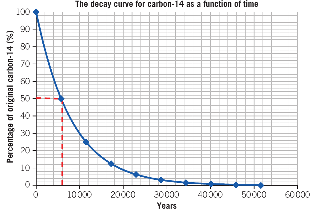
This decay curve demonstrates that:
- If 50% of the original carbon-14 remains, the object is 5,730 years old (one half-life)
- If 25% remains, the object is 11,460 years old (two half-lives)
- If 12.5% remains, the object is 17,190 years old (three half-lives)
Mathematical modelling of decay
The decay formula
The general formula for calculating radioactive decay is:
This equation can be used in two ways:
- Finding the final amount when you know the number of half-lives
- Finding the number of half-lives when you know the final amount
Worked Example: Carbon-14 Dating
Problem: A bone fragment from an archaeological dig has one-eighth of the original carbon-14 remaining. Carbon-14 has a half-life of 5,730 years. How old is the bone fragment?
Solution:
First, recognize that
Therefore, half-lives have elapsed.
Age of bone = years
Answer: The bone fragment is 17,190 years old.
Worked Example: Cobalt-60 Medical Source
Problem: A 10 g radioactive medical cobalt-60 source has an initial activity of 440 TBq and a half-life of 5.27 years. The source needs replacement when its activity decreases to of its initial value.
a) When will it need replacement? b) What will its activity be at that time? c) How many grams will remain?
Solution:
a) Time for replacement
Since , four half-lives have elapsed:
Time = years
b) Activity at replacement
Activity = TBq
c) Mass remaining
Mass remaining = g
Answers:
- The source will need replacement after 21.08 years
- Its activity will be 27.5 TBq
- Only 0.625 g will remain
Carbon-14 dating techniques
Carbon-14 dating works because living organisms constantly exchange carbon with their environment, maintaining a constant ratio of carbon-14 to carbon-12. When an organism dies, this exchange stops, and the carbon-14 begins to decay while carbon-12 remains stable. By measuring the ratio of carbon-14 to carbon-12, scientists can determine when the organism died.
Materials that can be dated
Radiocarbon dating can be applied to many materials containing organic carbon:
- Charcoal, wood, twigs, seeds
- Bones and shells
- Leather, peat, and soil
- Hair and pottery
- Pollen and wall paintings
- Corals and blood residues
- Fabrics, paper, parchment
- Resins and water samples
The wide variety of materials that can be dated with carbon-14 makes this technique invaluable for archaeology, anthropology, geology, and many other fields of study.
Medical applications
Technetium-99m: the medical workhorse
Technetium-99m is the most widely used radioactive isotope for medical diagnostic studies. Hospitals prefer short-lived isotopes because they minimize radiation exposure to patients.
Rather than using expensive particle accelerators, hospitals produce technetium-99m using a "radioactive cow" - a generator containing molybdenum-99 (the "mother" nuclide with a 67-hour half-life). As molybdenum-99 decays, it produces technetium-99m (the "daughter" nuclide with a 6.0-hour half-life):
The technetium-99m is extracted ("milking the cow") and used for medical imaging before it decays.
Why "Radioactive Cow"? The process of extracting daughter nuclides from a longer-lived parent isotope is called "milking" because it resembles milking a cow - the mother isotope continuously produces the useful daughter isotope, which is periodically harvested.
Activity and strength of radioactive sources
Definition of activity
Activity measures the strength of a radioactive source. It is defined as the number of nuclei that decay each second - essentially the rate of disintegrations.
The unit of activity is the becquerel (Bq), where:
Remembering Becquerels: Think of "Bq = Break per second" - becquerel measures how many atomic nuclei break (decay) per second.
Cobalt-60 decay and activity
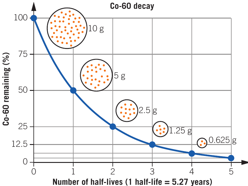
Cobalt-60 is a gamma-ray emitter with a half-life of 5.27 years. It is used for sterilising medical equipment and in external radiotherapy. Consider a medical source containing 10 g of cobalt-60:
- Initial activity: 440 TBq ( Bq)
- After one half-life (5.27 years): 5 g remains, activity = 220 TBq
- After two half-lives (10.54 years): 2.5 g remains, activity = 110 TBq
- After three half-lives (15.81 years): 1.25 g remains, activity = 55 TBq
Key Relationship: As the amount of radioactive material decreases, so does its activity. This has important implications for the working lifespan of medical equipment - the source must be replaced when activity drops too low to be effective.
Natural radioactivity on Earth
Sources of radiation
Since Earth formed 4,500 million years ago, two major mechanisms have produced natural radiation:
- Terrestrial radiation - from radioactive elements in Earth's crust
- Cosmic radiation - from space
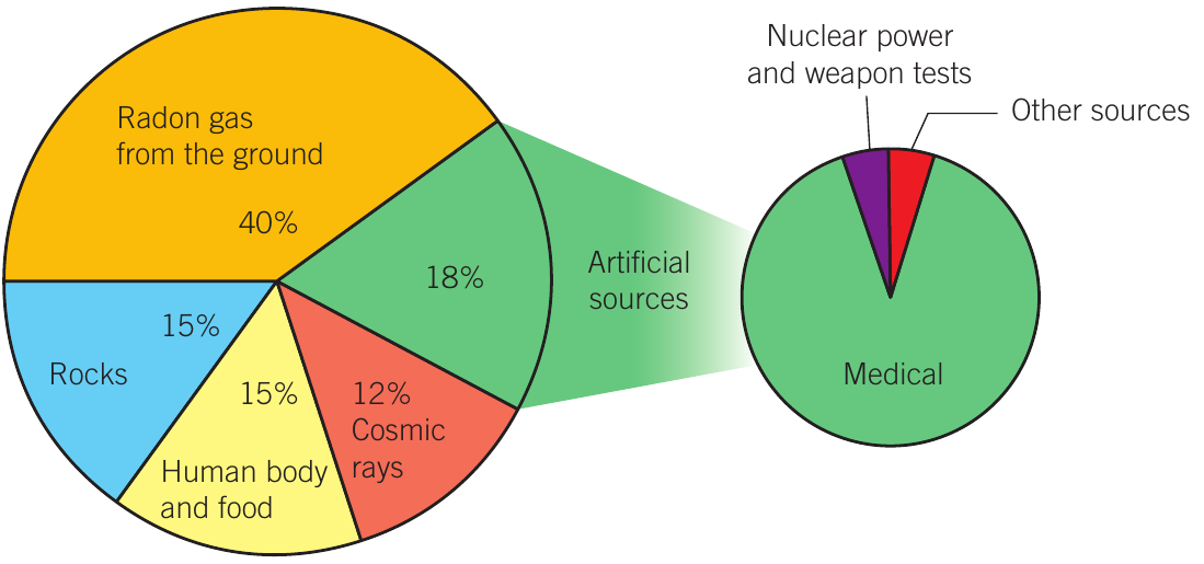
Approximately 82% of the average annual radiation that people receive comes from natural sources:
- Radon gas from the ground: 40%
- Rocks and soil: 15%
- Human body and food: 15%
- Cosmic rays: 12%
- Artificial sources (mainly medical): 18%
The majority of human radiation exposure is from natural sources that have existed throughout our evolution. Artificial sources, primarily medical procedures, contribute only about 18% of our total exposure.
Radioactivity in everyday life
We are constantly exposed to low levels of radiation from everyday items:
| Item | Radioisotope | Activity |
|---|---|---|
| 1 kg bananas | Potassium-40 | 100 Bq |
| 1 kg brazil nuts | Radium-226 | 250 Bq |
| Australian home (100 m²) | Radon-222 | 3 kBq |
| 70 kg adult human | Potassium-40 | 7 kBq |
| Smoke detector | Americium-241 | 30 kBq |
| Medical diagnosis | Fluorine-18 | 5 MBq |
| Medical therapy | Caesium-137 | 100 TBq |
Human radioactivity
Humans are naturally radioactive! A 70 kg person contains potassium-40, a gamma-ray emitter with a half-life of 1.25 billion years, producing approximately 7,000 disintegrations per second (7 kBq). This potassium is essential for proper body function and is obtained from food like bananas. This natural radioactivity has been present throughout human evolution.
Don't Fear the Banana! The radioactivity in bananas and other foods containing potassium is completely natural and harmless. Our bodies have evolved with this background radiation, and the potassium-40 is essential for nerve and muscle function.
Half-lives of common isotopes
| Isotope | Half-life |
|---|---|
| Uranium-238 | 4.5 billion years |
| Potassium-40 | 1.25 billion years |
| Carbon-14 | 5,730 years |
| Radium-226 | 1,600 years |
| Americium-241 | 460 years |
| Strontium-90 | 28 years |
| Iodine-131 | 8.1 days |
| Technetium-99m | 6.0 hours |
| Bismuth-214 | 20 minutes |
| Polonium-214 | 0.15 milliseconds |
When Earth formed 4.5 billion years ago, there was twice as much uranium-238 as exists now - exactly what we'd expect after one half-life has elapsed. This provides strong evidence for the age of our planet.
Key exam skills
Using the half-life equation effectively
The decay formula can be applied in two directions:
Direction 1: Given the number of half-lives, find the final amount
- Substitute the known values into the equation
- Calculate the result
Direction 2: Given the final amount, find the number of half-lives
- Express the fraction as a power of
- The exponent gives you the number of half-lives
Exam Strategy: Always identify what you're given and what you need to find before starting calculations. Write out the formula first, then substitute values carefully. Double-check whether you need to find or .
Key Points to Remember:
-
Radioactive decay is random - you cannot predict when an individual nucleus will decay, but you can predict the behaviour of large groups statistically
-
Half-life is constant - the half-life of a particular isotope never changes and is unaffected by external conditions like temperature or magnetic fields
-
The decay formula is - memorise this and understand each variable:
- = original amount (N-naught)
- = final amount (N-now)
- = number of half-lives
-
Activity measures decay rate - measured in becquerels (Bq), where 1 Bq = 1 disintegration per second
-
All decay curves have the same exponential shape - the only differences are the scale values on the axes
-
Half the Half - remember that each half-life reduces the amount by half again