Big O Notation and Classification of Algorithms Revision Notes for AQA A-Level Computer Science

Big O Notation and Classification of Algorithms

Introduction

An algorithm is a set of instructions that performs a specific task. Programs are built from algorithms, and these can range from just a few lines of code to millions of lines depending on the complexity of the problem being solved. For instance, a typical phone app contains around 100,000 lines of code, while the latest version of Microsoft Office uses approximately 45 million lines of code. This shows that there's usually a relationship between the size of the problem and the amount of code needed to solve it.

Understanding how to classify algorithms based on their efficiency is crucial when writing good code. This chapter explores how you can compare different algorithms by examining their complexity - specifically, how much time they take to run and how much memory they require. The method used to describe this is called Big O notation.

Classifying algorithms

When faced with a problem, programmers may develop different algorithms to provide a solution. One of the key objectives when writing code is to create an efficient solution. Efficiency is typically measured in two ways:

Time and space complexity

Time complexity refers to how long an algorithm takes to run compared to other algorithms. This is the main focus for A-level study and is what we typically mean when discussing algorithm efficiency.

Space complexity refers to how much memory an algorithm requires compared to other algorithms. While both are important, time complexity is usually the primary consideration.

infoNote

The critical factor when evaluating these measures is the input size (also called problem size). This is the number of parameters or values that the algorithm processes. As the input size grows, the performance characteristics of different algorithms become more apparent.

For example, a search routine designed for a small dataset with just a few values might not work efficiently on a larger dataset containing hundreds of values. The relationship between input size and algorithm performance is fundamental to understanding Big O notation.

lightbulbExample

Worked Example: Bubble Sort Analysis

Consider a bubble sort algorithm, which is generally inefficient because it must loop through the entire dataset repeatedly, comparing and swapping adjacent items on each pass.

The Problem: If there were a million items of data, the algorithm might need to make approximately $1,000,000^2$ comparisons - that's an enormous number of operations!

Basic Implementation: Here's how a basic bubble sort works in pseudocode:

For Loop1 = 1 To NumberOfItems - 1
    For Loop2 = 1 To NumberOfItems - 1
        'if the following name is smaller then swap
        If NameStore(Loop2) > NameStore(Loop2 + 1) Then
            SwapData = NameStore(Loop2)
            NameStore(Loop2) = NameStore(Loop2 + 1)
            NameStore(Loop2 + 1) = SwapData
        End If
    Next
Next

Improved Version: The algorithm can be improved by checking whether any swaps have occurred in each pass. If no swaps are made, the data is already sorted and no further iterations are needed:

Do
    SwapData = ""
    For Loop2 = 1 To CountTo
        If NameStore(Loop2) > NameStore(Loop2 + 1) Then
            SwapData = NameStore(Loop2)
            NameStore(Loop2) = NameStore(Loop2 + 1)
            NameStore(Loop2 + 1) = SwapData
        End If
    Next
    CountTo = CountTo - 1
Loop Until SwapData = ""

Key Insight: We need to analyse how algorithms respond to changes in input size to understand their true efficiency.

Functions

Before diving into Big O notation, we need to understand some mathematical concepts. Big O notation uses standard mathematical functions to describe algorithm complexity.

What is a function?

A function relates an input to an output. For example, $f(x) = x^2$ is a function. This means you take the input value $(x)$ and produce an output by squaring it.

The domain is the set of values that can possibly be input to a function. The codomain is the set of values that could possibly come out of the function. The range is the set of values that are actually produced by the function. The range will always be a subset of the codomain.

lightbulbExample

Worked Example: Understanding Function Components

For the function $f(x) = x^2$ :

The domain might be all real numbers
The codomain might be all real numbers
The range would be only non-negative real numbers (since squaring always produces a positive result or zero)

If $x = -3$ , then $f(-3) = (-3)^2 = 9$ If $x = 5$ , then $f(5) = 5^2 = 25$

Notice that both negative and positive inputs produce positive outputs, which is why the range only includes non-negative numbers.

Permutations and factorials

Another important concept for understanding Big O is permutations. Consider different ways items can be arranged:

A word with two letters has 2 permutations: 'to' can be 'to' or 'ot'
A word with three letters has 6 permutations: 'dog' can be 'dog', 'dgo', 'odg', 'ogd', 'gdo' or 'god'
A word with four letters has 24 permutations. The formula is: four ways to pick the first letter, then three ways to pick the second letter, then two ways to pick the third letter, and finally one way to pick the last letter: $4 \times 3 \times 2 \times 1 = 24$
A word with five letters has $5 \times 4 \times 3 \times 2 \times 1 = 120$ permutations

This is called the factorial function, denoted by $n!$ where $n$ is an integer. For our five-letter word, we write this as $5!$ , which equals $5 \times 4 \times 3 \times 2 \times 1 = 120$ .

infoNote

Factorials grow extremely rapidly. While $5! = 120$ seems manageable, $10! = 3,628,800$ and $20! = 2,432,902,008,176,640,000$ . This rapid growth is why algorithms with factorial complexity are considered intractable.

Big O notation

Big O notation is a method of describing the time complexity and space complexity of an algorithm. It examines the worst-case scenario and asks the question: how much slower will this code run if we give it 1,000 things to work on instead of 1?

For example, with a bubble sort that compared pairs of data items and swapped them if necessary, the algorithm might work quite quickly on a list of 10 items. But what if you asked it to sort a list of 1 million items?

chatImportant

Big O notation provides a measure of how the running time requirements grow as the input size increases. It calculates the upper bound - the maximum amount of time it would take to complete the algorithm. The notation refers to the order of growth, which measures how much more time or space it takes to execute the code as the input size increases.

The format uses a capital letter O followed by a function. All of the explanations below relate specifically to time complexity rather than space complexity.

Five main classifications

Big O notation uses five main classifications to describe algorithm efficiency:

O(1) - Constant time

Constant time means the algorithm will always execute in exactly the same amount of time regardless of the input size.

Accessing an array element is an example of $O(1)$ complexity. Each element in the array can be accessed directly by referring to its position. Whether there's one element or ten million elements in the array, it takes the same amount of time to access a single element.

infoNote

$O(1)$ doesn't necessarily mean the code runs quickly - it just means the execution time is constant regardless of input size. An $O(1)$ operation that takes 10 seconds will still take 10 seconds whether processing 1 item or 1 million items.

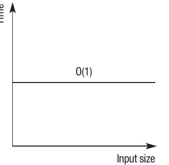
The graph shows that no matter how much the input size increases, the time taken to run the algorithm remains constant.

O(N) - Linear time

Linear time represents a direct proportional relationship between input size and runtime. If you input twice as much data, the algorithm will take twice as long to complete.

The relationship can be represented as $y = x$ , where every change in $x$ produces a corresponding change in $y$ . The linear relationship may be more complex - for example, $O(N)$ could be $y = 2x$ , which means that every change in $x$ would produce double this change in $y$ .

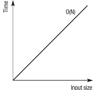
Looping through a list is an example of $O(N)$ because the code needs to access every element of the list. If you increase the size of the list, the time taken to complete the loop increases by a linear amount.

lightbulbExample

Worked Example: Linear Search

Consider searching through an unsorted array for a specific value:

For i = 0 To ArrayLength - 1
    If Array[i] = SearchValue Then
        Return i
    End If
Next
Return -1

Analysis:

Best case: The item is at the first position - $1$ comparison
Worst case: The item is at the last position or not present - $N$ comparisons
Average case: The item is somewhere in the middle - $N/2$ comparisons

Since we focus on worst-case scenarios, this algorithm has O(N) complexity.

O(N²) - Polynomial time

Polynomial time means the runtime increases proportionate to the square of the input size. To take a simplified example: if one item takes 1 second $(1^2)$ , then ten items would take 100 seconds $(10^2)$ , and 100 items would take 10,000 seconds $(100^2)$ . This can be expressed as $y = x^2$ .

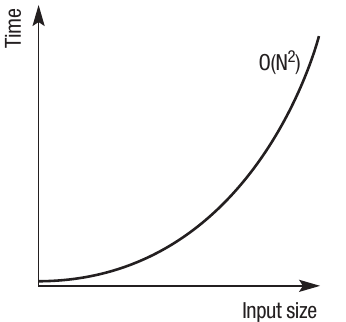
Iterative or nested statements such as bubble sorts and insertion sorts are examples of $O(N^2)$ complexity. The program has to go back through itself repeatedly with each iteration.

lightbulbExample

Worked Example: Nested Loop Analysis

For instance, in a bubble sort implemented with nested loops:

Private Sub btnSort_Click(ByVal sender As System.Object, ByVal e As System.EventArgs) Handles btnSort.Click
    Dim Loop1 As Integer
    Dim Loop2 As Integer
    Dim TempStore As String
    Dim RowsToSort As Integer
    
    RowsToSort = grdDataIn.RowCount - 2
    For Loop1 = 1 To RowsToSort - 1
        For Loop2 = 1 To RowsToSort - 1
            'compare each value in the table with the following value
            'changing the > operator will sort high to low
            If grdDataIn.Rows(Loop2).Cells(0).Value > grdDataIn.Rows(Loop2 + 1).Cells(0).Value Then
                'swap values to move larger values to later cells
                TempStore = grdDataIn.Rows(Loop2).Cells(0).Value
                grdDataIn.Rows(Loop2).Cells(0).Value = grdDataIn.Rows(Loop2 + 1).Cells(0).Value
                grdDataIn.Rows(Loop2 + 1).Cells(0).Value = TempStore
            End If
        Next
    Next
End Sub

Analysis: The nested loops mean the algorithm must process each item multiple times:

Outer loop runs approximately $N$ times
Inner loop runs approximately $N$ times for each outer loop iteration
Total operations: $N \times N = N^2$

This leads to quadratic growth in execution time.

O(2^N) - Exponential time

Exponential time means the runtime will double with every additional unit increase in the input size. To take a simplified example: one item might take 1 second, two items would take 2 seconds, three items would take 4 seconds, and so on. Ten items of data would take 512 seconds. This can be expressed as $y = 2^x$ , where $x$ is each individual item being input and $y$ represents the time taken.

chatImportant

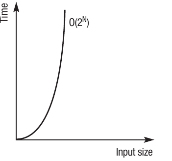
The time taken to process each input quickly becomes unworkable. Problems with an exponential order of growth are often referred to as intractable problems, which means they can't be solved with a computer in a reasonable time. We'll explore this more later in the chapter.

O(logN) - Logarithmic time

Logarithmic time uses an exponent to raise the value of a base number to produce a desired result. For example, with $y = \log_2 x$ , if $x = 8$ then $y$ must equal $3$ , because you multiply $2 \times 2 \times 2$ (or $2^3$ ) to get $8$ . In base ten, if $y = \log_{10} x$ and $x = 10,000$ , then $y$ equals $4$ , as $10 \times 10 \times 10 \times 10$ (or $10^4$ ) equals $10,000$ .

The efficiency of logarithmic algorithms is demonstrated by binary search. Binary search works by continually splitting the data in half until the item being searched for is found. It's called a binary search because it splits the data in two each time. This gives it a time complexity of $O(\log_2 N)$ , as each subsequent split of the data takes less time - only half the data is being searched.

lightbulbExample

Worked Example: Binary Search Efficiency

Here's how the number of comparisons scales with dataset size in binary search:

Table

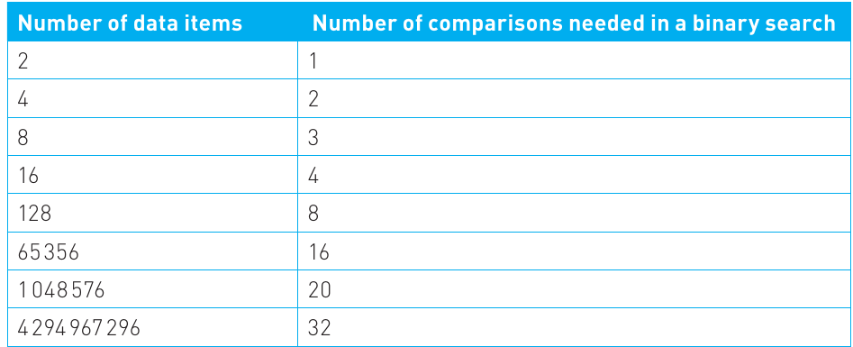
Analysis: The table shows that even with over 4 billion data items, a binary search only requires 32 comparisons!

Why is this so efficient?

Each comparison eliminates half of the remaining data
$2^{32} = 4,294,967,296$
Therefore, 32 divisions by 2 can handle over 4 billion items
Compare this to a linear search which would require up to 4 billion comparisons!

This demonstrates how efficiently logarithmic algorithms scale. Even large datasets can be searched with relatively few operations.

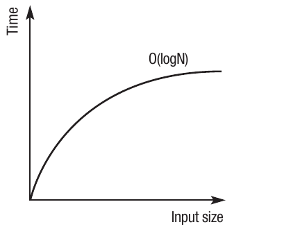
The graph shows the characteristic logarithmic curve - steep initial growth that gradually flattens as input size increases.

Comparing efficiencies

Big O notation helps you find the most efficient solution for your problem. It measures the upper bound, giving you an indication of how scalable your solution is - in other words, how efficient it will be as the input size increases.

bookmarkSummary

Efficiency Ranking (Most to Least Efficient):

O(1) algorithms scale the best, as they never take any longer to run regardless of input size
O(logN) algorithms are the next most efficient
O(N) algorithms are the next most efficient
O(N²) algorithms are polynomial and are considered to be the point beyond which algorithms start to become intractable. Note that the superscript number could be any value
O(2^N) algorithms are the least efficient and are considered intractable

Deriving the complexity of an algorithm

It's possible to determine the time complexity of an algorithm by examining its code structure. Here are some guidelines:

Simple operations - O(1):

An algorithm that requires no data and contains no loops or recursion, such as a simple assignment statement or comparison statement, will have a time complexity of $O(1)$

Single loops - O(N):

An algorithm that loops through an array, accessing each data item once, will have a time complexity of $O(N)$

Nested loops - O(N²):

An algorithm with inner and outer loops will be polynomial, with runtime increasing depending on the depth of the nesting and the number of loops. In this case it will be $O(N^2)$
The addition of a loop within the inner loop would alter the polynomial time to $O(N^3)$

Recursive algorithms - O(a^N):

An algorithm that uses recursion to call itself could have a time complexity of $O(a^N)$ , where a represents the base

infoNote

It's not always straightforward to work out the precise time complexity, as it may depend on how many times parts of the algorithm run based on the outcome of conditional statements. For example, with an If statement, part of the algorithm will only need to run if a condition is true. Therefore, the actual number of times some program code executes will depend on the data input to the algorithm when it's carried out.

When describing the complexity of a problem using Big O notation, the usual practice is to quote the worst-case scenario for the most efficient algorithm. However, when choosing a suitable algorithm, it's possible to make a comparison between the worst, best and average cases based on time complexity.

Common algorithm complexities

Here are some well-known algorithms and their time complexities:

Complexity	Algorithms
$O(1)$	Indexing an array
$O(\log N)$	Binary search
$O(N)$	Linear search of an array
$O(N^2)$	Bubble sort, Selection sort, Insertion sort
$O(2^N)$	Intractable problems

Tractable and intractable problems

A tractable problem is one that can be solved in polynomial time. In simple terms, this means the algorithm that solves the problem runs quickly enough for it to be practical to use on a computer.

Intractable problems are those which are theoretically possible to solve but cannot be solved within polynomial time. The problem may be solvable if the input size is small, but as soon as the input size increases, it's considered impractical to try and solve it on a computer.

The travelling salesman problem

A classic example of an intractable problem is the travelling salesman problem, which has been studied by mathematicians and computer scientists for over 100 years:

A salesman has to travel between a number of cities
The distance between each pair of cities is known
He must visit each city just once and then return to his start point
He must calculate the shortest route

lightbulbExample

Worked Example: The Complexity of the Travelling Salesman Problem

The Challenge: On the face of it, there may be a simple solution to this problem, particularly if there are only a small number of cities to visit. However, as the number of cities increases, the permutations of routes grow at a much faster rate.

Real-World Scale: There are many similar problems that involve calculating distances between pairs of points. For example, some analyses look at points on a circuit board to optimise data transmission. The time complexity of such problems is typically concerned with the worst-case scenario, so must consider thousands of points.

Current Limitations: To date, algorithms have been created that can calculate the actual shortest distance between around 85,000 pairs of points. These algorithms have a very large time complexity that goes well beyond polynomial time and are therefore considered intractable.

Heuristic algorithms

Faced with intractable problems, programmers often produce heuristic algorithms. A heuristic approach accepts that the perfect solution is not possible, so a solution that provides an incomplete or approximate result is considered preferable to no solution at all. Often this involves ignoring certain complex elements of the problem or accepting a solution that is not optimal.

chatImportant

Heuristics use 'rules of thumb' and therefore cannot guarantee accurate results for every possible set of inputs. Instead, they produce results that may be accurate for common uses of the program, but less accurate when the program is used with less likely inputs. The objective with a heuristic algorithm is to produce an acceptable solution in an acceptable time frame, where the optimum solution would simply take too long.

For example, several heuristic solutions have been developed for the travelling salesman problem that theoretically enable millions of cities to be considered. None of these compare every possible pair of cities, so they don't create an actual solution. Instead, they produce an approximate solution which may be very accurate. Estimates suggest some of these methods produce results that may be within 5% degree of accuracy of the optimum solution.

Unsolvable problems

Unsolvable problems are those which will never be solved, regardless of how much computing power is available, either now or in the future, regardless of how much time is given to solve it.

The halting problem is an example of a problem that has been proven to be unsolvable. In simple terms, the halting problem asks whether it's possible to write a program to determine if a program will finish running for a particular set of inputs.

infoNote

The question was devised by Alan Turing in the 1930s, asking whether it would be possible to write a computer program to solve the halting problem. The conclusion is that the problem is unsolvable - it has been proven that it cannot be done.

The halting problem is considered to be one of the first unsolvable problems ever identified and has led to the discovery of many other unsolvable problems. This area of computing has led to a general acceptance that there are some problems which:

Simply cannot be solved by computers (unsolvable problems)
Can theoretically be solved by computers but it is not possible within a reasonable time frame (intractable problems)

Remember!

bookmarkSummary

Key Points to Remember:

Algorithm efficiency is measured primarily by time complexity (how long it takes to run) and space complexity (how much memory it uses)
Big O notation describes algorithm complexity using mathematical functions, focusing on how performance changes as input size increases
Five main complexity classes from most to least efficient: $O(1)$ constant, $O(\log N)$ logarithmic, $O(N)$ linear, $O(N^2)$ polynomial, $O(2^N)$ exponential
Tractable problems can be solved in polynomial time, making them practical for computer solution, while intractable problems cannot be solved in reasonable time despite being theoretically solvable
Heuristic algorithms provide approximate solutions to intractable problems by accepting "good enough" results rather than perfect solutions, while unsolvable problems like the halting problem can never be solved by any computer program

Big O Notation and Classification of Algorithms (AQA A-Level Computer Science): Revision Notes