The Turing Machine (AQA A-Level Computer Science): Revision Notes
The Turing Machine
Introduction to the Turing machine
The Turing machine is a theoretical model of computation that was created by British mathematician Alan Turing in 1936. At the time, Turing was investigating what became known as the 'decision problem' - essentially, he wanted to determine whether it was theoretically possible to solve any mathematical problem within a finite number of steps when given specific inputs.
What makes the Turing machine particularly remarkable is that it was conceived as a purely theoretical concept rather than an actual physical machine. Turing created a mathematical model that could perform any algorithm, and in doing so, he essentially established a framework for understanding what is computable. This work predated microprocessors and modern computing as we know them today by several decades.
Although the Turing machine was originally just a theoretical idea, scientists have since built physical machines based on Turing's model, and software simulations of Turing machines are widely available. The fundamental concepts behind the Turing machine continue to underpin our understanding of computation and what computers can and cannot do.
Components of a Turing machine
A Turing machine consists of three essential components that work together to perform computations. Understanding these components is crucial to grasping how the machine operates.
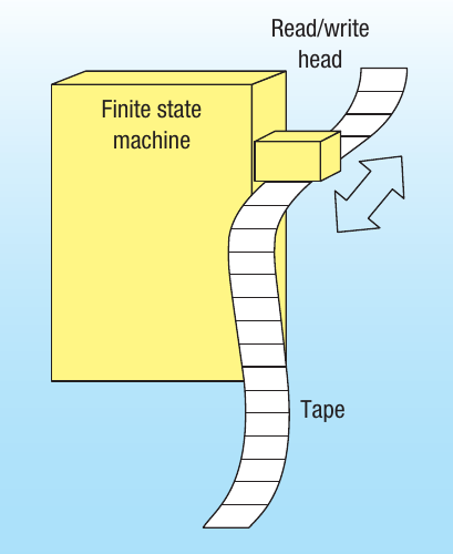
The finite state machine (FSM) acts as the control unit of the Turing machine. This is any device that stores its current status and can change that status based on input it receives. You can think of it as the "brain" of the machine that makes decisions about what to do next. The FSM is used as a conceptual model for designing and describing computational systems.
The tape provides the memory for the Turing machine. Unlike computer memory which has finite capacity, the Turing machine's tape is theoretically infinite in length. The tape is divided into individual sections called cells, with each cell able to hold a single symbol. The tape essentially serves the same purpose as RAM in a modern computer, storing both the input data and any intermediate results during computation.
Each cell on the tape contains a symbol from the machine's alphabet. This alphabet consists of the acceptable symbols (such as characters or numbers) that the particular Turing machine can work with. Typically, the alphabet for a Turing machine includes binary digits (0s and 1s) and a special blank symbol (often represented as □), though any symbols could potentially be used.
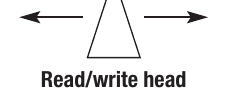
The read/write head is the mechanism that interacts with the tape. This theoretical device can perform three key operations: it can read what symbol is currently in a cell, it can write a new symbol into the cell (effectively overwriting the current contents), and it can move left or right along the tape to access different cells. The head can only move one cell at a time, ensuring that every cell is accessible through sequential movement.
How the Turing machine operates
Understanding how these components work together helps you see why the Turing machine serves as such a powerful model of computation. The machine operates through a series of discrete steps, following rules that determine its behaviour.
At any given moment, the machine is in a particular state. The start state is where the machine begins its operation - this is the initial state before any computation has taken place. As the machine processes information, it transitions between different states according to its programming.
The read/write head examines the symbol in the current cell. Based on both this symbol and the machine's current state, the machine follows its transition rules to determine what happens next. These rules specify three things: what symbol (if any) to write in the current cell, which direction to move the head (left or right by one cell), and what state to transition to next.
The machine continues this process - read, write, move, change state - repeatedly until it reaches a special halting state. The halting state stops the Turing machine's operation, indicating that the computation is complete and the final output has been produced. The machine can also halt if the entire input has been processed according to its rules.
The halting state is critical to every Turing machine. Without it, the machine would continue processing indefinitely without producing a final result. This concept is directly related to the famous "halting problem" in computer science - determining whether a program will eventually stop or run forever.
Interestingly, despite being invented before computers existed, this model closely resembles how modern computers work. The tape represents memory, the read/write head is analogous to memory addressing mechanisms, and moving through the tape by reading and executing instructions is very similar to how a computer executes a program. The key difference is that real computers have finite memory, whereas the Turing machine's tape is theoretically infinite.
Representing programs in Turing machines
To make a Turing machine solve a particular problem, you need to define several key elements that together specify the "program" the machine will follow. These elements constitute the machine's programming and determine exactly what computation it will perform.
Every Turing machine program requires:
- A start state that defines where the machine begins operation at the start of the program
- A halting state that will stop the program when the computation is finished
- An alphabet listing all acceptable symbols that can appear in the cells
- Movement rules defining the head's ability to move left or right so it can read from and write to different cells
- A transition function that specifies what should be written at each cell and whether to move left or right based on the current state and the input symbol being read
The transition function is essentially the algorithm encoded as a set of rules. It tells the machine exactly what to do in every possible situation (combination of current state and input symbol). Without a complete transition function, the machine wouldn't know how to proceed when it encounters certain inputs.
State transition diagrams
One common way to represent the transition function of a Turing machine is through a state transition diagram. These diagrams provide a visual representation that is similar to the finite state machine diagrams you may have studied previously.
In a state transition diagram:
- Each state is represented as a circle with the state name inside (such as S0, S1, SH)
- The starting state is indicated by an arrow pointing to it from outside the diagram
- The halting state is shown as a double circle to distinguish it from other states
- Transitions between states are shown as arrows connecting the circles
- Each transition arrow is labelled with the format "input/output,movement"
For example, a label of "1/1,R" means: if the current input symbol is 1, write a 1 to the tape, and move right (R). Similarly, "□/0,R" means: if the input is a blank symbol (□), write a 0, and move right. Some states may have self-loops (arrows that start and end at the same state), which means the machine stays in that state under certain conditions.
The state transition diagram provides a clear visual overview of the machine's behaviour. By following the arrows and reading the labels, you can trace through exactly what the machine will do with any given input.
Instruction tables
An alternative way to represent the same information is through an instruction table (also called a transition table). This tabular format can be easier to read for some people and is particularly useful when documenting Turing machine programs in written form.
An instruction table has five columns:
| State | Read | Write | Move | Next state |
|---|
- State: The current state the machine is in
- Read: The symbol currently being read from the tape
- Write: The symbol to write to the tape (which may be the same as what was read)
- Move: The direction to move the head (R for right, L for left)
- Next state: The state to transition to after this operation
Each row in the table represents one transition rule. The table contains one row for every possible combination of state and input symbol, ensuring the machine knows what to do in every situation it might encounter.
Both state transition diagrams and instruction tables represent exactly the same information - they're just different formats. You may find one or the other easier to understand depending on the complexity of the Turing machine and your personal preference.
Worked example: odd parity generator
Worked Example: Odd Parity Generator
Let's look at a concrete example to see how a Turing machine works in practice. This example implements an odd parity generator - an algorithm that ensures a binary string contains an odd number of 1s.
The algorithm works as follows:
- The starting point is the left-most non-blank symbol in the binary string
- As the machine scans through the digits, it counts how many 1s it encounters
- If there is an even number of 1s, the machine adds a 1 at the end to make the total odd
- When a blank is reached, if there are already an odd number of 1s, the machine adds a 0 to maintain the odd count
- The program then halts
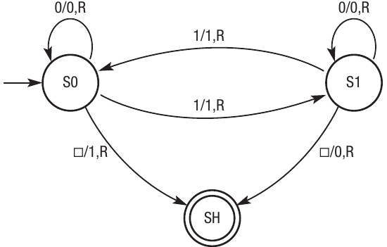
Here's how we can represent this using a state transition diagram that shows two states (S0 and S1) plus the halting state (SH):
| State | Read | Write | Move | Next state |
|---|---|---|---|---|
| S0 | □ | 1 | R | SH |
| S0 | 0 | 0 | R | S0 |
| S0 | 1 | 1 | R | S1 |
| S1 | □ | 0 | R | SH |
| S1 | 0 | 0 | R | S1 |
| S1 | 1 | 1 | R | S0 |
Step-by-step execution trace:
Let's trace through an example where the input tape contains "1 1 1 0 0". The machine starts in state S0 and the read/write head begins at the first 1.
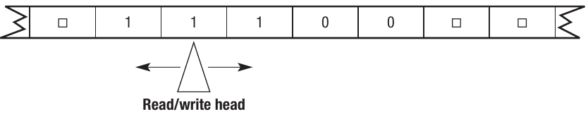
Step 1: The current input symbol is 1 and we're in state S0. According to the transition rules, we write a 1 to the tape, move right, and change to state S1.
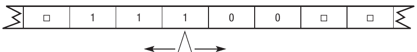
Step 2: Now we're in state S1 reading another 1. The rule "1/1,R" for state S1 tells us to write 1, move right, and transition back to state S0.
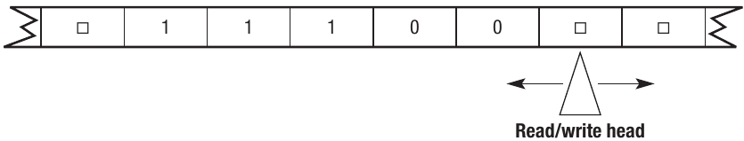
Step 3: We continue this process: reading a 1 in S0 transitions us to S1, then we read a 0 which keeps us in S1. The next 0 also keeps us in S1 according to the "0/0,R" rule.
Step 4: Eventually we reach a blank symbol (□) while in state S1. The transition rule "□/0,R" tells us to write a 0, move right, and transition to the halting state SH.
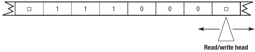
Result: The machine now stops, and the final tape contains "1 1 1 0 0 0" - the original input plus an added 0 to maintain an odd number of 1s (three 1s remains odd).
Alternative notation
Transition rules can also be written using function notation with the Greek letter δ (delta):
For the odd parity generator, the complete set of rules would be:
- (S0, □) = (SH, 1, R)
- (S0, 0) = (S0, 0, R)
- (S0, 1) = (S1, 1, R)
- (S1, □) = (SH, 0, R)
- (S1, 0) = (S1, 0, R)
- (S1, 1) = (S0, 1, R)
The blank symbol □ is commonly represented in notation, though some sources may use other symbols like B. Similarly, left and right movement might be shown as L and R, or as arrow symbols (← →).
Universal machine
At a theoretical level, you can use a Turing machine to solve any problem that is computable. However, there's a practical limitation: each individual process or computation requires its own specific Turing machine to perform it. If you have a large program with many different operations, you would need many different Turing machines.
You could think of this as a black box model where you define the inputs, the process to be carried out, and the output. For example:
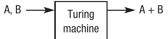
If you want to add two numbers A and B, you need one Turing machine designed specifically for addition.
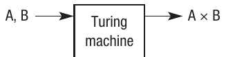
If you want to multiply A and B, you need a completely different Turing machine designed for multiplication.
For any complex program, having to build and manage separate Turing machines for every operation would quickly become impractical. This is why Alan Turing developed the concept of a universal machine - a single machine that can simulate any other Turing machine.
The universal machine is one of the most significant concepts in computer science. Rather than defining each individual process within a separate machine, the universal machine takes two types of input:
- A description of all the individual Turing machines needed to perform the required calculations (essentially, the programs)
- All the inputs required for those calculations (the data)
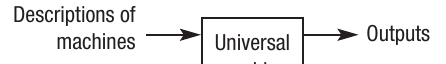
Think of the universal machine as a collection of individual Turing machines all linked together, capable of taking any input and performing any calculation defined by any of its component machines.
In practical terms, the universal machine stores everything on a single tape. One block of cells contains the instructions (the descriptions of what Turing machines to simulate), and another block contains the data (the inputs to process). The result is a machine that can simulate any number of Turing machines with their corresponding inputs and produce a range of different outputs depending on what's needed.
This is actually one of the earliest forms of the stored program concept that you may have studied in other chapters. The idea that both instructions and data can be stored together in the same memory is one of the key principles of modern computing. Even though the universal machine was devised as long ago as 1936, well before modern computers existed, it demonstrates this fundamental concept. Modern computers work in essentially the same way - programs and data are both stored in memory and processed together.
Because Turing machines break down processes into small individual steps, the universal machine concept mirrors other computational techniques you've encountered, such as decomposition, where large problems are broken down into smaller, more manageable sub-problems until a programmable solution can be found.
The concept of the Turing machine and the universal machine is also closely connected to the idea of computable problems. If it's possible to describe a Turing machine that can solve a problem, then it will be possible to write an algorithm to solve it on a real computer. This relationship defines the theoretical limits of what computers can and cannot do.
Remember!
Key Points to Remember:
-
The Turing machine is a theoretical model created by Alan Turing in 1936 to investigate whether mathematical problems could be solved algorithmically. It consists of three components: a finite state machine, an infinite tape divided into cells, and a read/write head.
-
The machine operates by reading symbols from the tape, writing symbols to the tape, and moving left or right one cell at a time based on transition rules. It continues until reaching a halting state, at which point the computation is complete.
-
Turing machines can be represented using state transition diagrams (showing states as circles and transitions as labelled arrows) or instruction tables (showing state, read, write, move, and next state in columns). Both methods represent the same transition function.
-
The universal machine solves the problem of needing separate Turing machines for different operations. It can simulate any Turing machine by reading descriptions of machines along with input data from the same tape, demonstrating the stored program concept fundamental to modern computing.
-
Despite being conceived before computers existed, the Turing machine model closely resembles how modern computers work, with the tape acting as memory, the read/write head as memory addressing, and transition rules as instructions. The key difference is that real computers have finite memory whilst the Turing machine's tape is theoretically infinite.