Price, Income, and Cross Elasticities (AQA A-Level Economics): Revision Notes

Price, Income, and Cross Elasticities

The meaning of elasticity

When economists study markets, they need to understand how responsive one variable is to changes in another. This is where the concept of elasticity becomes essential.

Elasticity measures how much one variable changes in proportion to a change in another variable. Think of it as measuring the sensitivity or responsiveness between two economic factors.

For example, imagine a product's price increases by 5%. If consumers reduce their purchases by more than 5%, we say demand is elastic — it responds strongly to price changes. However, if consumers only reduce their purchases by less than 5%, demand is inelastic — it responds weakly to price changes. When the percentage change in quantity exactly matches the percentage change in price, we have unit elasticity of demand.

Types of elasticity

Economists focus on three main types of demand elasticity:

• Price elasticity of demand — measures how quantity demanded responds to price changes
• Income elasticity of demand — measures how quantity demanded responds to income changes
• Cross elasticity of demand — measures how demand for one good responds to price changes in another good

Formulae for calculating elasticities

Each type of elasticity has its own formula:

Price elasticity of demand (PED):

$\text{PED} = \frac{\text{\% change in quantity demanded}}{\text{\% change in price}}$

Income elasticity of demand (YED):

$\text{YED} = \frac{\text{\% change in quantity demanded}}{\text{\% change in income}}$

Cross elasticity of demand (XED):

$\text{XED} = \frac{\text{\% change in quantity of good A demanded}}{\text{\% change in price of good B}}$

Price elasticity of demand

Price elasticity of demand measures how responsive consumers are to price changes for a particular good. It tells us the extent to which quantity demanded changes when price changes.

Sometimes this is called 'own price' elasticity to distinguish it from cross elasticity, which measures responsiveness to changes in the price of a different good.

Infinite and zero price elasticity of demand

At the two extremes of price elasticity, we find demand curves with constant elasticity values at all points.

A perfectly elastic demand curve is horizontal. This shows infinite price elasticity (PED = ∞). Even the tiniest price increase causes quantity demanded to fall to zero. Conversely, any price decrease would cause quantity demanded to rise to infinity.

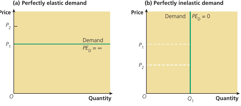
A perfectly inelastic demand curve is vertical. This shows zero price elasticity (PED = 0). When price falls (for example, from P₁ to P₂), the quantity demanded remains completely unchanged. Price changes have no effect whatsoever on quantity demanded.

The five demand curves you need to know

There are five key types of demand curve based on their elasticity:

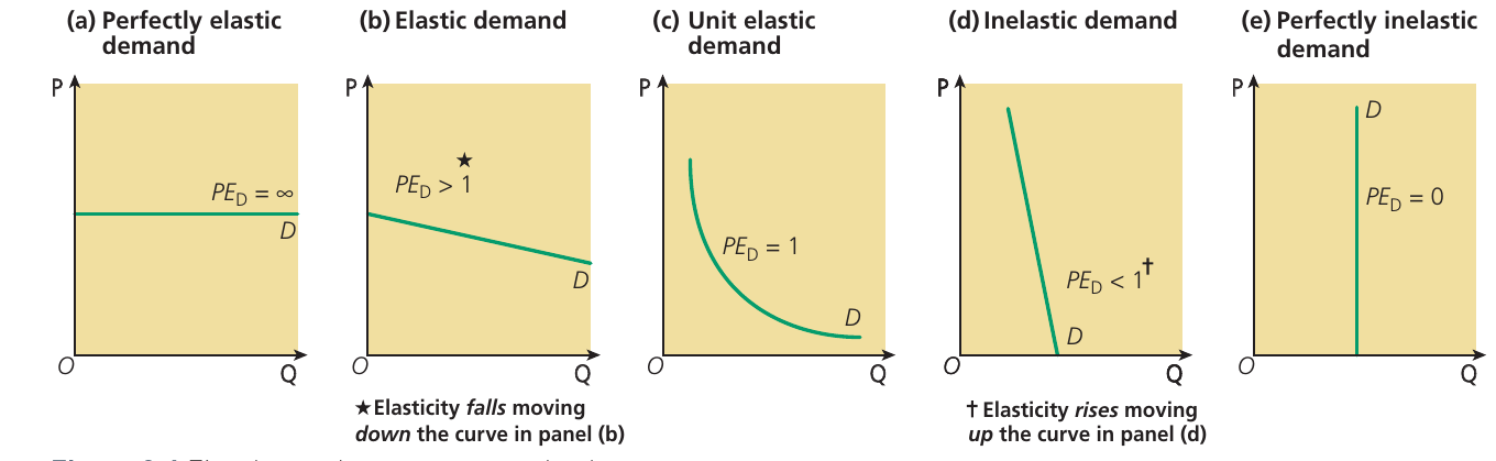
• Perfectly elastic demand (PED = ∞) — horizontal line
• Elastic demand (PED > 1) — relatively flat, downward-sloping curve
• Unit elastic demand (PED = 1) — curved line (rectangular hyperbola)
• Inelastic demand (PED < 1) — relatively steep, downward-sloping curve
• Perfectly inelastic demand (PED = 0) — vertical line

Factors determining price elasticity of demand

Several key factors influence how elastic or inelastic demand will be for a particular product.

Substitutability

This is the most important determinant of price elasticity. When close substitutes are readily available for a product, consumers can easily switch to alternatives if the price rises. This makes demand highly elastic.

Conversely, when no substitutes or only poor substitutes exist, demand tends to be inelastic. Consumers have limited alternatives, so they continue buying even when prices increase.

Percentage of income

Goods and services that take up a large proportion of household income tend to have more elastic demand than those representing only a small fraction of income.

When items account for only a tiny portion of income, consumers barely notice price changes, especially for goods they rarely purchase. People are less sensitive to price movements for these items.

However, for 'big-ticket' purchases like new cars or overseas holidays that consume a significant portion of income, consumers are much more responsive to price changes. They pay close attention to prices and adjust their purchasing decisions accordingly.

Necessities or luxuries

There's a common belief that demand for necessities is price inelastic, while demand for luxuries is elastic. However, this statement requires careful consideration.

When no obvious substitute exists, demand for a luxury good may actually be inelastic. At the other extreme, demand for particular types of basic foodstuff can be elastic if other staple foods are available as substitutes.

The 'width' of the market definition

The broader the market definition under consideration, the lower the price elasticity of demand.

For example, demand for bread from a particular bakery is likely more elastic than demand for bread from all bakeries. This is because bread from other bakeries provides close substitutes for bread from just one bakery.

If we widen the market definition further, demand for bread produced by all bakeries will be more elastic than demand for food as a whole. Different foods can substitute for each other, but at the level of all food, there are fewer alternatives available.

Time

The time period in question significantly affects price elasticity of demand.

Short run refers to the time period when at least one factor of production is fixed and cannot be varied. Long run refers to the time period when no factors are fixed and all factors of production can be varied.

For many goods and services, demand is more elastic in the long run than in the short run. This is because it takes time for consumers to respond to price changes.

In other circumstances, the response might be greater in the short run than the long run. A sudden rise in petrol prices might cause motorists to economise on petrol use for a few weeks before getting used to the higher price and drifting back to their old motoring habits.

Case study: elasticity and tobacco taxation

Various studies have calculated the price elasticity of demand for cigarettes across different groups in society, including young and old smokers, and men and women.

The research also found greater price responsiveness among younger people, with an average price elasticity of -1.43 for teenagers, -0.76 for young adults, and -0.32 for adults.

These studies reveal that adult smokers have an average price sensitivity between -0.50 (men) and -0.34 (women), with lower-income groups showing greater price sensitivity.

Follow-up considerations:

1. The formula PED = percentage change in quantity demanded / percentage change in price is used for these calculations.
2. Income elasticity and cross elasticity of demand are the other two types besides price elasticity.
3. Adult smokers may be less responsive than teenagers because of stronger addiction and higher disposable incomes. Teenagers are more price-conscious and haven't developed such strong habits.
4. These elasticity statistics between zero and -1 indicate inelastic demand, which is significant for governments. Tax increases on cigarettes will raise substantial revenue because consumption doesn't fall proportionately. This helps fund public health initiatives.

Price elasticity of demand, total consumer expenditure and firms' total revenue

There's a useful rule for determining the general nature of elasticity between two points on a demand curve without using the formula.

• If total consumer expenditure increases in response to a price fall, demand is elastic
• If total consumer expenditure decreases in response to a price fall, demand is inelastic
• If total consumer expenditure remains constant in response to a price fall, demand is neither elastic nor inelastic (i.e. elasticity = unity, or since the demand curve slopes downwards, elasticity = minus unity or -1)

Consider the elastic demand curve shown below:

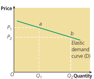
At price P₁, total consumer expenditure is shown by the rectangle bounded by P₁, point a, Q₁ and the origin O. When price falls to P₂, the consumer expenditure rectangle changes to the area bounded by P₂, point b, Q₂ and O. The second rectangle is clearly larger than the first, so total consumer expenditure increases following a price fall. This confirms the demand curve is elastic.

Unit elastic demand and expenditure

When demand has unit elasticity, total expenditure remains unchanged following a price change. This special case occurs when the demand curve is a rectangular hyperbola — a specific curved line where the proportionate change in quantity demanded exactly equals the proportionate change in price.

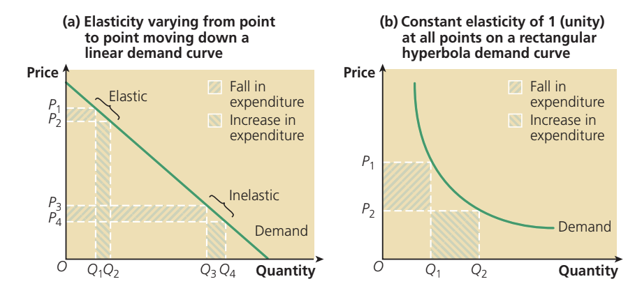
For a rectangular hyperbola demand curve, consumer expenditure remains constant whether price rises or falls. The elasticity equals unity (or -1 considering the negative relationship) at all points on this curve. Mathematicians call this special curve shape a rectangular hyperbola because whenever price falls, the proportionate change in quantity demanded exactly matches the proportionate change in price, keeping total expenditure constant.

Income elasticity of demand

Income elasticity of demand measures how responsive demand is to changes in income. It shows the extent to which quantity demanded for a good changes when consumer income changes.

The nature of income elasticity depends on whether the good is classified as a normal good or an inferior good.

When disposable income increases, a demand curve shifts rightwards, but only if the good is a normal good (where demand increases as income rises). However, some goods are inferior goods, for which demand decreases as income increases. An increase in income actually shifts the demand curve for an inferior good leftwards.

Categories of normal goods

Normal goods can be further divided into superior goods (or luxuries) and necessities.

Superior goods have an income elasticity of demand greater than +1. Although the quantity demanded of a normal good always rises with income, it rises by a greater percentage for superior goods like luxury cars.

Necessities have an income elasticity lying between zero and +1. Demand for basic goods or necessities like shoe polish rises by a smaller percentage than the increase in income.

Application example

The UK's income elasticity for overseas holidays is +1.6. This tells us that overseas holidays are a superior good (luxury) for UK consumers. When UK incomes rise by 10%, demand for overseas holidays rises by 16%. This makes sense because holidays abroad are a discretionary purchase that people spend more on proportionately as they become wealthier.

Cross elasticity of demand

Cross elasticity of demand (or cross-price elasticity of demand) measures how the demand for one good responds to changes in the price of another good.

The cross elasticity between two goods or services indicates the nature of the demand relationship between them. There are three possibilities:

• Complementary goods (or goods in joint demand)
• Substitutes (or competing goods)
• An absence of any discernible demand relationship

Complementary goods

Cars and petrol (or diesel fuel) are complementary goods — they're in joint demand. A significant increase in fuel prices, such as the 30.7% increase in petrol prices in the year to March 2022, affects the demand for cars, though the effect may not be large.

By contrast, private car travel and bus travel are substitute goods. A significant increase in the cost of running a car causes some motorists to switch to public transport, provided bus fares don't rise by a similar amount.

For most demand relationships between two goods, cross elasticities are inelastic rather than elastic, both when the goods are in joint demand and when they are substitutes.

Negative cross elasticity: complementary goods

Complementary goods (or goods demanded together) have negative cross elasticities of demand. A rise in the price of one good leads to a fall in demand for the other good.

Positive cross elasticity: substitute goods

By contrast, the cross elasticity of demand between two goods which are substitutes for each other is positive. A rise in the price of one good causes demand to switch to the substitute good whose price hasn't risen, so demand for the substitute increases.

For example, a new bicycle and a new motor scooter are substitutes for each other. If the cross elasticity of demand for a new bicycle with respect to the price of a motor scooter is +0.4, this tells us that a 10% increase in the price of new motor scooters will lead to a 4% increase in demand for new bicycles as consumers switch between these two types of private transport.

Zero cross elasticity: no relationship

If we select two goods at random — for example, pencils and suitcases — the cross elasticity of demand between them will be zero. When there's no discernible demand relationship between two goods, a rise in the price of one good has no measurable effect upon the demand for the other. The cross elasticity of demand is zero, unless both items make up an important part of household expenditure.