Costs (Edexcel A-Level Economics A): Revision Notes
Costs
Introduction to costs facing firms
When firms make decisions about how much to produce, they must carefully consider how production costs change with different output levels. Understanding the relationship between costs and output is essential for making profitable business decisions.
Costs vary depending on the time period being considered and how factors of production are combined. This note explores different types of costs, how they behave in both the short run and long run, and why some firms benefit from producing on a large scale whilst others do not.
Understanding cost behaviour is fundamental to business decision-making. Firms need to know how costs respond to changes in output to determine optimal production levels and maintain profitability.
Short run and long run
To understand how costs behave, we first need to distinguish between two important time periods: the short run and the long run.
The short run is the period during which a firm can only vary some of its factors of production. Typically, labour is considered a variable factor in the short run because firms can hire more workers, increase overtime, or reduce working hours relatively quickly. However, capital (such as machinery, factories, or equipment) is treated as a fixed factor because it takes considerable time to install new machinery or build new factories.
The long run is the period during which a firm can vary all its factors of production, including both labour and capital. In the long run, firms have complete flexibility to change their scale of operations by adjusting all inputs.
Key Distinction:
The difference between short run and long run isn't about calendar time—it's about flexibility. The short run is any period where at least one factor remains fixed, whilst the long run is when all factors can be varied. For a small bakery, the long run might be months; for an oil refinery, it could be years.
This distinction is crucial because it affects how costs respond to changes in output and which production decisions are available to the firm.
The law of diminishing marginal productivity
A fundamental principle governing short-run production is the law of diminishing marginal productivity. This law states that if a firm increases the input of one variable factor (such as labour) whilst holding other factors fixed (such as capital), it will eventually experience diminishing additional output from each extra unit of the variable factor.

Worked Example: Programmers and Computers
Consider a practical example. Imagine an office with 10 computers and 10 programmers:
-
Adding the 11th programmer: Output might increase slightly, as workers could take coffee breaks at different times and maintain continuous work.
-
Adding the 12th programmer: This might also add some extra output.
-
Adding more programmers beyond this point: If the firm keeps adding programmers without increasing the number of computers, each additional worker will contribute less and less to total output.
-
The 20th worker: Might add nothing at all, being unable to access a computer.
This demonstrates diminishing marginal productivity in action.
The law of diminishing marginal productivity is a short-run concept because it relies on the assumption that some factors of production remain fixed. In the long run, the firm could purchase more computers to accommodate additional programmers, eliminating the constraint.
Types of costs in the short run
Because some inputs cannot be varied in the short run, we can categorise costs into different types:
Total fixed costs (TFC) are costs that do not change with the level of output produced. These might include rent on a factory, lease payments on machinery, or contracted salaries. The firm must pay these costs even if it produces nothing at all.
Total variable costs (TVC) are costs that vary directly with the level of output. These typically include costs of raw materials, wages paid to casual staff, and operating costs such as electricity for running machinery. As output increases, variable costs increase because more inputs are needed.
Sunk costs are a particular type of fixed cost that cannot be recovered if the firm closes down. For example, if a firm has already paid for advertising or has commissioned specialist equipment, these expenditures cannot be recouped.
The Fundamental Cost Relationship:
This simple equation is the foundation for understanding all other cost measures. Total costs always consist of the sum of fixed costs (which don't change) and variable costs (which change with output).
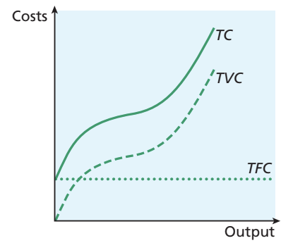
The diagram above shows how these costs relate to each other. Total fixed costs remain constant at all output levels (shown as a horizontal line). Total variable costs start at zero when output is zero and increase as output rises. Total costs start at the level of fixed costs (when output is zero) and then increase parallel to variable costs.
Average and marginal costs
Firms often need to understand costs on a per-unit basis, which is where average costs become important. There are several types of average costs to consider:
Average total cost (ATC) measures the total cost per unit of output produced. It is calculated as:
Average total cost is particularly important because it varies with output levels, primarily due to the law of diminishing marginal productivity. As output initially increases, average total cost typically falls. However, as diminishing returns set in, average total cost begins to rise.
Average fixed cost (AFC) measures fixed costs per unit of output:
Since fixed costs don't change, average fixed cost continuously falls as output increases. The fixed costs are simply spread over more and more units of output.
Average variable cost (AVC) measures variable costs per unit of output:
Average variable cost typically follows a U-shape, initially falling and then rising as diminishing returns affect productivity.
Marginal cost (MC) is the cost of producing one additional unit of output. It measures how much total cost changes when output increases by one unit:
Marginal cost is crucial for decision-making because firms often decide whether to produce more by comparing the marginal cost against the marginal revenue (additional revenue from selling one more unit). If marginal revenue exceeds marginal cost, producing the additional unit increases profit.
Worked example: calculating costs
Worked Example: Calculating Different Cost Measures
Let's examine how these different cost measures relate to each other using numerical data:
| Output (000 units per week) | Fixed costs (TFC) | Total variable cost (TVC) | Total cost (TC) = (2) + (3) | Average total cost (SATC) (4)/(1) | Marginal cost (MC) Δ(4)/Δ(1) | Average variable cost (AVC) (3)/(1) | Average fixed cost (AFC) (2)/(1) |
|---|---|---|---|---|---|---|---|
| 1 | 225 | 85 | 310 | 310 | 65 | 85 | 225 |
| 2 | 225 | 150 | 375 | 187.5 | 60 | 75 | 112.5 |
| 3 | 225 | 210 | 435 | 145 | 90 | 70 | 75 |
| 4 | 225 | 300 | 525 | 131.25 | 175 | 75 | 56.25 |
| 5 | 225 | 475 | 700 | 140 | 395 | 95 | 45 |
| 6 | 225 | 870 | 1,095 | 182.5 | - | 145 | 37.5 |
Key Observations from the Data:
This table illustrates several important patterns:
-
Fixed costs remain constant at £225 per week regardless of output—demonstrating the nature of fixed costs.
-
Variable costs rise steeply as output increases, particularly after 4,000 units, reflecting diminishing marginal productivity.
-
Average total cost initially falls from 310 to 131.25 as output increases from 1,000 to 4,000 units, but then begins to rise again. This happens because average total cost is composed of average variable cost and average fixed cost. Whilst average fixed cost continuously falls (spreading fixed costs over more units), average variable cost eventually rises due to diminishing returns. The combination creates the characteristic U-shape of the average total cost curve.
-
Marginal cost demonstrates important behaviour: After the third unit, marginal cost rises sharply, jumping from 90 to 175 and then to 395. This steep increase reflects the impact of diminishing marginal productivity.
Graphing short-run costs
Understanding the graphical representation of short-run costs helps visualise the relationships between different cost measures.
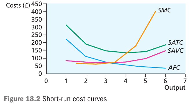
The diagram above shows the four key short-run cost curves:
The short-run marginal cost (SMC) curve is U-shaped, initially falling and then rising steeply. This reflects how the cost of producing each additional unit first decreases (as the firm becomes more efficient) and then increases (as diminishing returns set in).
The short-run average total cost (SATC) curve is also U-shaped. Initially, average total cost falls as both average fixed costs decline and the firm benefits from better resource utilisation. However, as diminishing marginal productivity takes effect, average total cost eventually rises.
The short-run average variable cost (SAVC) curve has a shallow U-shape, reflecting the changing efficiency of variable input usage.
The average fixed cost (AFC) curve slopes continuously downwards because fixed costs are spread over increasing amounts of output.
Critical Relationship Between Marginal and Average Costs:
The marginal cost curve always cuts both the average variable cost curve and the average total cost curve at their minimum points. This occurs because of a mathematical property: when the marginal cost is below the average cost, it pulls the average down. When marginal cost exceeds average cost, it pushes the average up. Therefore, average cost must be at its minimum when marginal cost equals average cost.
Understanding the Marginal-Average Relationship: The Cricket Analogy
Think of this like calculating a cricket player's batting average:
-
If a player scores less than their current average in their next innings (marginal performance below average), their average falls.
-
If they score more than their current average (marginal performance above average), their average rises.
-
The average only stays constant when the new score exactly equals the existing average.
This same principle explains why marginal cost intersects average cost at the average's minimum point.
Another important feature is that the average variable cost curve gets closer to the average total cost curve at higher output levels. This happens because the difference between them is average fixed cost, which becomes smaller as output increases.
Costs in the long run
In the long run, firms can adjust all their factors of production, including capital. This flexibility means firms can choose the most appropriate scale of production for their expected output level.
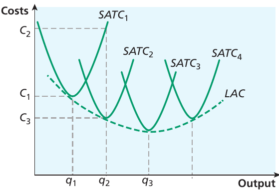
The diagram above illustrates the relationship between short-run and long-run costs. Each U-shaped curve (, , , ) represents the short-run average total cost for a different capital stock level. If a firm wants to produce output level , it would install capital corresponding to , allowing production at cost . For output , the firm would choose , achieving cost .
The long-run average cost (LAC) curve forms an envelope that just touches each short-run average total cost curve. This envelope shows the lowest possible average cost for any output level when the firm can freely vary all inputs. The LAC curve represents the planning curve that firms use when deciding what scale of operation to adopt.
The LAC Curve and SATC Curves:
Notice that the LAC curve doesn't necessarily touch each SATC curve at its minimum point. For example, to produce output , the firm operates at the minimum of (point A). However, to produce output , the firm operates to the left of the minimum of (point B). This reflects the fact that different scales of production are optimal for different output levels.
Economies of scale
One of the most important reasons firms benefit from being large is the existence of economies of scale. Economies of scale occur when an increase in a firm's scale of production leads to lower long-run average costs. Understanding why economies of scale arise helps explain firm size and market structure in different industries.
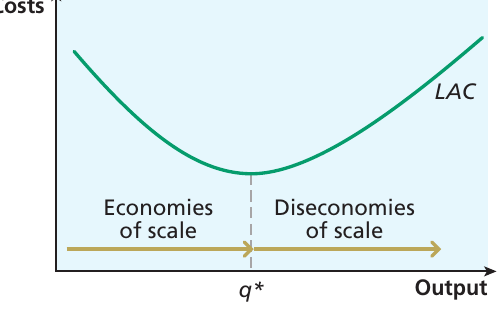
The diagram above shows the classic U-shaped long-run average cost curve. On the left side, the curve slopes downward, indicating economies of scale. As output increases beyond , the curve slopes upward, indicating diseconomies of scale. The output level represents an important point we'll discuss later.
Sources of economies of scale
Several factors contribute to economies of scale:
Technology
Many production technologies favour large-scale operations. Consider shipping: a large vessel can transport proportionally more cargo than a small ship relative to its surface area. Similarly, large barrels hold more wine relative to their surface area than small barrels. This physical property means larger operations can be more efficient.
Moreover, certain capital equipment is specifically designed for large-scale production and would not be economically viable at small output levels. A car production line, for instance, cannot feasibly operate at very low volumes. This creates indivisibilities in the production process that favour larger firms.
The importance of fixed costs
Many industries involve substantial overhead expenditures that don't vary with output levels. Once a factory is built, its cost remains the same regardless of how much is produced in it. Research and development spending is another overhead that may only be viable when a firm reaches a certain size.
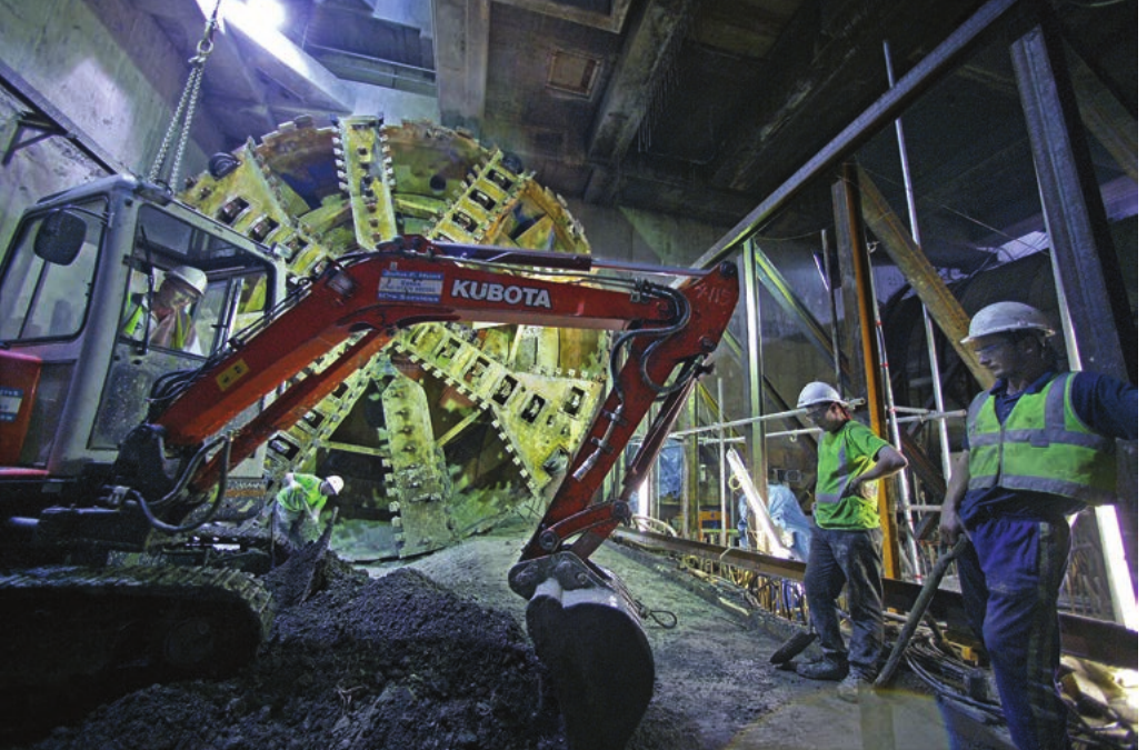
Worked Example: The Channel Tunnel and Fixed Costs
Consider the Channel Tunnel project. The construction costs were enormous compared to the ongoing costs of running trains through the tunnel. This substantial fixed cost element creates significant economies of scale.
Key Insight: The largest firm in such markets can always produce at lower average cost than smaller firms, potentially creating what economists call a natural monopoly—a situation where only one firm can viably serve the market.
Natural Monopolies:
Natural monopolies arise in industries with such substantial economies of scale that competition becomes unsustainable. Examples include:
- Railway networks
- Electricity distribution
- Telecommunications infrastructure (in some cases)
In these industries, the most efficient outcome is to have a single large producer rather than multiple smaller ones.
Management and marketing
As firms expand, they can benefit from management economies of scale. A certain number of managers are required to oversee production processes. As the firm grows, the volume of output increases faster than the need for additional management, allowing management costs to be spread over larger production volumes. Larger firms can also manage more efficiently by specialising management roles and improving coordination.
Similarly, marketing costs may not rise proportionally with firm size. A television advertising campaign or marketing budget represents a substantial fixed cost element that larger firms can spread over greater sales volumes, reducing average cost.
Finance and procurement
Large firms often enjoy financial economies of scale by accessing capital on more favourable terms than smaller firms. Banks and investors may view large established firms as lower risk, offering them better interest rates or easier access to financing. This financial advantage reinforces the market position of larger firms and makes it harder for smaller competitors to become established.
Additionally, purchasing economies of scale arise when large firms negotiate better terms with suppliers by buying raw materials, energy, and transport services in bulk. Suppliers may offer volume discounts or preferential terms to their largest customers.
Technical economies of scale
Technical economies of scale emerge when increasing size allows improved technical efficiency. This might involve adopting more advanced production methods, investing in better technology, or achieving higher capacity utilisation rates.
Diseconomies of scale
However, firms cannot grow indefinitely without encountering problems. Diseconomies of scale occur when increases in the scale of production lead to higher long-run average costs.
As organisations become very large, management can become more difficult. Coordination, communication, and control become increasingly challenging. Bureaucracy may increase, decision-making may slow down, and motivation problems may arise. Workers in very large organisations might feel disconnected from the firm's goals, reducing productivity.
The Minimum Efficient Scale (MES):
These management challenges mean that beyond a certain size, average costs may begin to rise. The output level at which long-run average cost stops falling is called the minimum efficient scale (MES). This represents the smallest scale of production at which a firm can minimise its long-run average costs.
External economies of scale
The economies of scale discussed so far are internal economies of scale—they arise from the expansion of an individual firm. However, firms can also benefit from external economies of scale, which arise from the expansion of the entire industry.
When an industry expands, several beneficial developments may occur:
- A pool of skilled labour develops as workers acquire industry-specific skills
- Educational institutions may begin offering relevant training courses, reducing individual firms' training costs
- Specialist suppliers and support services emerge to serve the industry
- Infrastructure improvements may occur to support the industry's needs
Worked Example: External Economies in the Web Design Industry
The growth of the web design industry created a pool of skilled designers and developers that individual firms could recruit from. As the sector expanded, colleges began offering web design courses, further increasing the availability of skilled workers.
Result: This benefited all firms in the industry, not just the largest ones. External economies of scale can be represented as a downward shift of the entire LAC curve rather than a movement along it.
Productive efficiency
When a firm operates at the lowest point on its long-run average cost curve, producing at the minimum efficient scale, it achieves productive efficiency. At this point, the firm has chosen the optimal combination of factors of production and produces the maximum possible output from those inputs. This represents the most cost-effective production level in the long run.
Shape of the long-run average cost curve
The U-shaped long-run average cost curve shown earlier represents one common pattern, but LAC curves can take various shapes depending on industry characteristics and technology.
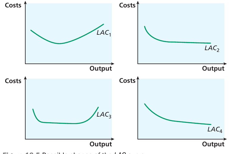
The diagram above shows four different possible shapes for long-run average cost curves:
shows the typical U-shape, with clear economies of scale initially, followed by diseconomies of scale.
displays continuous economies of scale that eventually flatten out, showing constant returns to scale. This pattern might occur in industries where diseconomies of scale are limited.
exhibits an extended flat section in the middle, indicating a wide range of output over which constant returns to scale prevail. After initial economies of scale, the firm can operate efficiently across a broad range of outputs before diseconomies emerge.
shows perpetually declining average costs, suggesting economies of scale continue across all relevant output ranges. This pattern characterises natural monopoly situations where the largest firm always has a cost advantage.
The actual shape of the LAC curve depends on:
- The specific industry's technology
- The importance of fixed costs
- How quickly management difficulties emerge with size
- The nature of production processes
Economies of scope
Whilst this note focuses on costs related to a single product, it's worth noting that some firms produce multiple products and may benefit from economies of scope. These occur when producing several different products together is more cost-effective than producing them separately.
Worked Example: Nestlé and Economies of Scope
Nestlé produces hundreds of different products ranging from instant coffee to baby milk powder, mineral water, ice cream, and pet food.
Cost Advantage: The company can share certain functions across all these products—such as finance, accounting, human resources, and marketing departments—without needing separate departments for each product line.
Result: This sharing of resources across a range of products reduces average costs for each individual product.
Key Concepts to Remember
Key Points to Remember:
-
The short run is when at least one factor of production is fixed, whilst the long run is when all factors can be varied.
-
The law of diminishing marginal productivity explains why adding more variable inputs whilst holding fixed inputs constant eventually produces smaller increases in output, causing marginal cost to rise in the short run.
-
Cost relationships are crucial: , and the marginal cost curve always cuts both average variable cost and average total cost curves at their minimum points.
-
Economies of scale arise from various sources including technology, fixed costs, management efficiency, finance, and procurement, causing the LAC curve to slope downwards initially.
-
The minimum efficient scale represents the output level at which long-run average cost stops falling, and firms achieve productive efficiency when operating at this point.