Perfect Competition Revision Notes for Edexcel A-Level Economics A

Perfect Competition

Perfect competition is a theoretical market structure that serves as an important benchmark in economic analysis. It represents an ideal form of market organisation where, under specific conditions, resources are allocated in the most efficient way possible for society. While perfect competition rarely exists in its pure form in the real world, understanding this model helps economists evaluate and compare other market structures.

infoNote

Although perfect competition is largely theoretical, it provides economists with a valuable framework for understanding how markets work and for comparing real-world market structures against an ideal benchmark.

The model of perfect competition

Perfect competition is a form of market structure that produces allocative and productive efficiency in long-run equilibrium. The model is based on strict assumptions that, if fulfilled, would ensure the best possible allocation of resources for society as a whole.

Assumptions of perfect competition

Perfect competition operates under six key assumptions that define how this market structure functions. Each assumption plays a crucial role in determining the behaviour of firms and the outcomes for the market.

Profit maximisation

Firms operating in perfect competition aim to maximise their profits. This might initially seem like firms are acting purely in self-interest without considering consumers. However, the pursuit of profit by firms and utility maximisation by consumers actually ensures that the market operates effectively. It is this self-interested behaviour that drives the market towards efficient outcomes.

Many participants

A fundamental assumption of the model is that there are numerous buyers and sellers in the market. This means that no individual trader—whether buyer or seller—is large enough to influence the market price on their own. The market price is determined by the collective interaction of all participants in the market.

From the sellers' perspective, this assumption implies that economies of scale are limited within the industry. If the minimum efficient scale is small relative to overall market demand, then no single firm can grow large enough to gain significant market influence. This prevents any one firm from becoming dominant and keeps the market competitive.

Homogeneous product

In perfect competition, the product is homogeneous, meaning that buyers view all products in the market as identical. There is no brand loyalty or product differentiation—consumers see one firm's product as a perfect substitute for another's.

chatImportant

The homogeneous product assumption is critical because it eliminates brand loyalty. If consumers saw products as different, firms could charge premium prices and gain market power, undermining the competitive nature of the market.

This assumption reinforces the previous point about many participants. If there were brand loyalty or product differentiation, a firm could become more popular than others and potentially charge a premium price. By ruling out this possibility, the model ensures that no individual seller can influence the selling price of the product.

No barriers to entry or exit

Firms must be free to join the market if they perceive it to be profitable, and they can exit from the market without hindrance. This assumption becomes particularly important when considering the long-run equilibrium towards which the market will tend.

The absence of barriers means that if existing firms in the market are making attractive profits, new firms will be able to enter freely. Conversely, if firms are making losses, they can leave the market without incurring additional costs. This free entry and exit mechanism is crucial for the long-run adjustment process.

Perfect knowledge

All participants in the market have perfect information about trading conditions. Buyers always know the prices that firms are charging, enabling them to purchase goods at the cheapest possible price. Similarly, firms are aware of product quality and cannot charge prices above the market level, as they will attract no customers.

Traders also possess full awareness of market conditions, allowing them to respond quickly to any changes. While this assumption may seem unrealistic, the growth of the internet and price comparison websites has made it easier for consumers to access information. This technological development has made the assumption of perfect knowledge more plausible in some modern markets, potentially increasing the number of markets that behave more like price takers.

infoNote

The rise of internet shopping and price comparison websites has brought some real-world markets closer to the perfect knowledge assumption. Consumers can now instantly compare prices across multiple sellers, making it harder for firms to charge above market price.

No externalities

Externalities are costs or benefits that affect third parties not directly involved in a transaction. In perfect competition, externalities are ruled out to explore the characteristics of the model in its purest form. This allows economists to focus on how the market operates when only the direct participants are affected by transactions.

Perfect competition in the short run

The firm as a price taker

Given the assumptions outlined above, an important implication emerges for individual firms operating in perfect competition. No individual trader can influence the price of the product. This means that a firm is a price taker—it must accept whatever price is set in the market as a whole.

As a price taker, the firm faces a perfectly elastic demand curve for its product. The diagram below illustrates this situation. The market price is set at $P_1$ , and the firm cannot sell at any other price. If the firm tries to set a price above $P_1$ , it will sell nothing because buyers are fully aware of the market price and know there is no quality difference between products offered by different firms. Since buyers have perfect information, they will not purchase at a higher price when they can buy identical products elsewhere at the market price.

What this also implies is that the firm can sell as much output as it wishes at the prevailing market price. There is no incentive for the firm to set a price below $P_1$ because it can already sell unlimited quantities at that going price. Thus, all firms charge the same price, $P_1$ .

chatImportant

Critical relationship in perfect competition: For a price-taking firm, average revenue (AR) and marginal revenue (MR) are both equal to price (P). This is because the firm can sell any quantity at the market price, so the revenue from each additional unit equals the price.

$AR = MR = P$

This is why demand curves for perfectly competitive firms are labelled as $AR = MR$ .

An important technical point arises from this situation. A firm that can sell as much output as it wants at the prevailing market price is a price taker. This means that average revenue and marginal revenue are the same. Average revenue equals price because if the firm charges the same price to all buyers, then average revenue equals price. Marginal revenue is also equal to price for the same reason. This is why diagrams of perfectly competitive firms label the demand curve as $AR = MR$ , which is also equal to price.

The firm's short-run supply decision

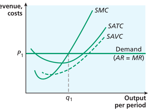
If the firm can sell as much as it likes at the market price, how does it decide how much to produce? To maximise profits, a firm needs to set output at a level where marginal revenue equals marginal cost ( $MR = MC$ ). The diagram below illustrates this rule by adding the short-run cost curves to the demand curve.

If the market price were to change, the firm would react by changing its output level, but always choosing to supply output at the level where $MR = MC$ . This suggests that the short-run marginal cost (SMC) curve represents the firm's short-run supply curve. In other words, it shows the quantity of output that the firm would supply at any given price.

However, there is one important qualification to this statement. If the price falls below short-run average variable cost (SAVC), the firm's best decision will be to exit from the market, as it will be better off just incurring its fixed costs rather than continuing to produce. Therefore, the firm's short-run supply curve is the SMC curve above the shut-down point where it intersects SAVC. For the industry as a whole, the short-run supply curve is the horizontal sum of the supply curves of all individual firms.

Industry equilibrium in the short run

One crucial question that has not yet been examined is how the market price is determined. To answer this, it is necessary to consider the industry as a whole. A conventional downward-sloping demand curve represents consumer preferences in the market.

On the supply side, the industry supply curve is formed by adding up the supply curves of each firm operating in the market. If you add up the supply curves of each firm (their individual marginal cost curves above SAVC), the result is the industry supply curve. The price will then adjust to the point where demand and supply intersect, establishing equilibrium for the industry. The firms in the industry will collectively supply the equilibrium quantity of output, and the market will be in equilibrium.

The firm in short-run equilibrium

The previous analysis seems to describe a well-balanced situation, with price adjusting to equate market demand and supply. However, the question remains as to why this is described as merely short-run equilibrium. The key to understanding this lies in examining the position facing an individual firm in the market.

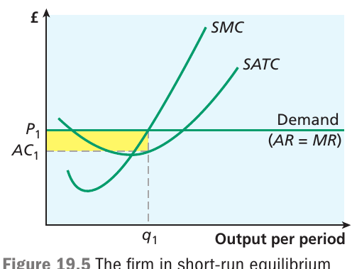
The diagram below returns to the position of an individual firm in the market. The firm maximises profits by accepting the price $P_1$ as set in the market and producing up to the point where $MR = MC$ , which occurs at output level $q_1$ .

At this point, the firm's average revenue (which equals price) is greater than its average cost (which is $AC_1$ at this level of output). The firm is thus making supernormal profits at this price, shown as the shaded area on the graph. Remember that 'normal profits' are included in average cost, so the amount of supernormal profit being made is calculated by multiplying the difference between average revenue and average cost by the quantity sold.

infoNote

Calculating supernormal profit:

$\text{Supernormal profit} = (AR - AC) \times Q$

where $AR$ is average revenue (price), $AC$ is average cost, and $Q$ is quantity produced. This appears as the shaded rectangular area on the diagram.

This is where the assumption about freedom of entry becomes crucial. If firms in this market are making profits above opportunity cost (supernormal profits), the market is generating more attractive returns than other markets in the economy. This will prove attractive to other firms, which will seek to enter the market. The assumption states that there are no barriers to prevent them from doing so.

The adjustment process

This process of entry will continue for as long as firms are making supernormal profits. However, as more firms join the market, the position of the industry supply curve (which is the sum of the supply curves of an ever-larger number of individual firms) will be affected. As the industry supply curve shifts to the right, the market price will fall. At some point, the price will have fallen to such an extent that firms are no longer making supernormal profits, and the market will stabilise.

chatImportant

The long-run adjustment mechanism:

If firms make supernormal profits → new firms enter → supply shifts right → price falls → profits return to normal
If firms make losses → firms exit → supply shifts left → price rises → profits return to normal

This entry and exit process continues until all firms make only normal profits in long-run equilibrium.

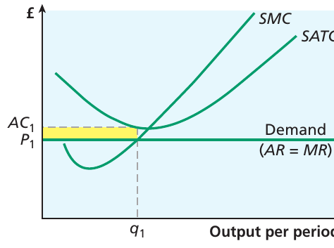
Conversely, if the price were to fall even further, some firms would make losses (where average cost exceeds price). These firms would choose to exit from the market, and the process would go into reverse. Price would be expected to stabilise such that the typical firm in the industry is making only normal profits.

The diagram below shows a situation where a firm tries to maximise profit by setting $MR = MC$ , but discovers that its average cost exceeds the price. The firm makes losses shown by the shaded area. In the long run, this firm will choose to leave the market. As this and other firms exit, the market supply curve shifts to the left, and the equilibrium price will drift upwards until firms are again making normal profits.

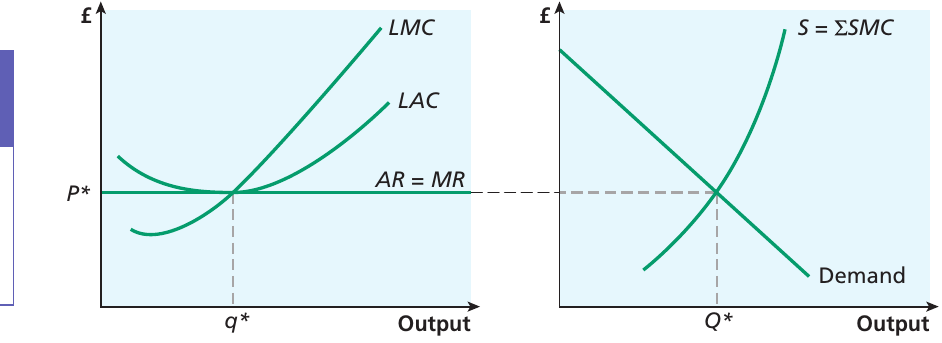
Perfect competition in long-run equilibrium

The diagram below shows the situation for a typical firm and for the industry as a whole once long-run equilibrium has been reached. At this point, firms no longer have any incentive to enter or exit the market. The market is in equilibrium, with demand equal to supply at the going price. The typical firm sets marginal revenue equal to marginal cost to maximise profits, producing at the output level $q^*$ and making only normal profits.

The long-run supply curve

Suppose there is an increase in demand for this product. Perhaps everyone becomes convinced that the product is genuinely health-promoting, so demand increases at any given price. This disturbs the market equilibrium, and the question is whether (and how) equilibrium can be restored.

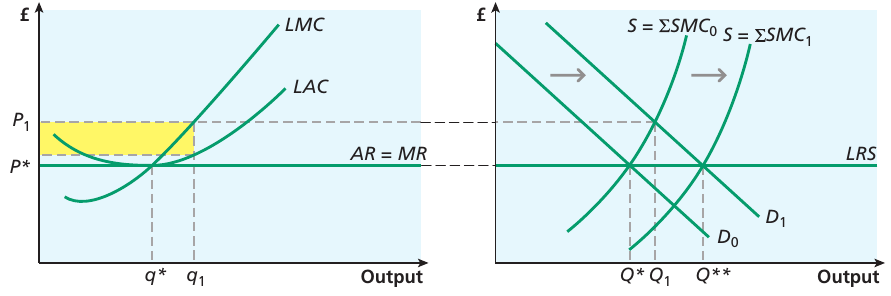
The diagram below reproduces the long-run equilibrium position from the previous diagram. In the initial position, market price is at $P^*$ , the typical firm is in long-run equilibrium producing $q^*$ , and the industry is producing $Q^*$ . Demand was initially at $D_0$ , but with increased popularity of the product it has shifted to $D_1$ .

lightbulbExample

Worked Example: How Markets Adjust to Increased Demand

Initial situation: Market in long-run equilibrium at price $P^*$ , industry output $Q^*$ , firms making normal profits.

Step 1 - Demand shock: Demand increases from $D_0$ to $D_1$

Step 2 - Short-run response: Price rises to $P_1$ , existing firms increase output to $q_1$ , industry output rises to $Q_1$ . Firms now make supernormal profits (shaded area).

Step 3 - Long-run adjustment: Supernormal profits attract new firms → entry of new firms shifts supply right → price falls back to $P^*$

Final equilibrium: Price returns to $P^*$ , but industry output is now higher at $Q^{**}$ . More firms are in the market, each producing $q^*$ , all making normal profits again.

In the short run, this pushes the market price up to $P_1$ for the industry. Existing firms have the incentive to supply more output as market price increases, so they move along their short-run supply curves. In the short run, a typical firm starts to produce $q_1$ output. The combined supply of all firms then increases to $Q_1$ .

However, at the higher price $P_1$ , the firms start making supernormal profits (shown by the shaded area in the left panel). Under the assumptions underpinning perfect competition, firms have perfect knowledge of market conditions, so they know that firms in the market are making supernormal profits. Furthermore, there are no barriers to entry that prevent new firms from joining the market. The fact that the product is homogeneous simplifies entry further.

This means that in time, more firms will be attracted into the market, pushing the short-run industry supply curve to the right. This process will continue until there is no further incentive for new firms to enter the market—which occurs when the price has returned to $P^*$ , but with increased industry output at $Q^{**}$ . In other words, the adjustment in the short run is borne by existing firms, but the long-run equilibrium is reached through the entry (or exit) of new firms.

This suggests that the industry long-run supply curve (LRS) is horizontal at the price $P^*$ , which is the minimum point of the long-run average cost curve for the typical firm in the industry. The LRS shows that in long-run equilibrium under perfect competition, the curve representing the typical firm in the industry is horizontal at the minimum point of the long-run average cost curve.

infoNote

The horizontal long-run supply curve reflects the fact that in perfect competition, the price always returns to the minimum point of long-run average cost. The market can supply any quantity at this price in the long run through entry and exit of firms, not through changes in price.

It is worth noting that if firms face different cost conditions, the LRS may slope upwards. This could happen because some firms face more favourable environments than others. Perhaps their location confers some advantage because they are closer to the market or to raw materials. This would allow some firms to survive for longer if the market price falls. In this case, as price falls, the least efficient firms would exit from the market until the marginal firm just makes normal profits. The most efficient firms in the market would still be able to make some supernormal profits even in long-run equilibrium, and it is only the marginal firm that just breaks even.

Efficiency under perfect competition

Having reviewed the characteristics of the long-run equilibrium of a perfectly competitive market, it is worth considering what is so beneficial about such a market in terms of productive and allocative efficiency.

Productive efficiency

For an individual market, productive efficiency is reached when a firm operates at the minimum point of its long-run average cost curve. Under perfect competition, this is indeed a feature of the long-run equilibrium position. Productive efficiency is therefore achieved in the long run—but not in the short run, when a firm is not necessarily operating at minimum average cost.

In long-run equilibrium under perfect competition, firms produce at the lowest point on their long-run average cost curve. This means they are producing at the minimum efficient scale, using resources as efficiently as possible from a production standpoint. There is no wastage of resources, and firms cannot reduce their average costs any further by changing their scale of operation.

infoNote

Productive efficiency condition:

$P = \text{minimum } LAC$

where $LAC$ is long-run average cost. This means firms are producing at the lowest possible cost per unit.

Allocative efficiency

For an individual market, allocative efficiency is achieved when price is set equal to marginal cost. Again, the process by which supernormal profits are competed away through the entry of new firms into the market ensures that price equals marginal cost within a perfectly competitive market in long-run equilibrium.

This outcome is significant because it means that the price consumers pay exactly reflects the marginal cost of producing the last unit. Resources are being allocated according to consumer preferences—society is producing the combination of goods and services that consumers most desire. There is no deadweight loss, and society's welfare is maximised.

infoNote

Allocative efficiency condition:

$P = MC$

This ensures that the value consumers place on the last unit (shown by price) equals the cost of producing it (marginal cost). Resources are being allocated efficiently according to consumer preferences.

It is important to note that firms set price equal to marginal cost even in the short run, so allocative efficiency is a feature of perfect competition in both the short run and the long run.

Dynamic efficiency

Perfect competition is not conducive to fostering dynamic efficiency. Dynamic efficiency refers to efficiency over time, particularly relating to innovation and technological progress. When firms only make normal profits, they do not have surplus funds available for investment in research and development or innovation.

chatImportant

The dynamic efficiency critique:

Perfect competition's major weakness is its lack of dynamic efficiency. Because firms earn only normal profits in long-run equilibrium, they have no surplus funds for:

Research and development
Innovation and new product development
Investment in new technologies
Improvements to production processes

This absence of supernormal profits means perfectly competitive firms cannot drive long-term economic progress through innovation.

In long-run equilibrium, perfectly competitive firms earn just enough to cover their opportunity costs. They have no spare resources to invest in developing new products, improving production processes, or adopting new technologies. This lack of funds for innovation is a significant limitation of perfect competition.

Some economists, such as Friedrich von Hayek, have argued that supernormal profits serve as the foundation for investment by firms in new technologies, research and development, and innovation. If supernormal profits are always competed away, as happens under perfect competition, firms cannot undertake these activities. Similarly, Joseph Schumpeter contended that only in monopoly or oligopoly markets can firms afford to undertake research and development.

X-inefficiency

The intensity of competition in a perfectly competitive market makes it unlikely that there will be X-inefficiency. X-inefficiency occurs when firms fail to minimise their costs—perhaps because management becomes complacent or because the organisational structure is inefficient.

In perfect competition, firms need to be rigorous in keeping costs down if they are to survive in the market. Any firm that allows X-inefficiency to creep in will find its costs rising above those of its competitors. With price determined by the market and all firms selling at the same price, a firm with higher costs will be unable to cover them and will make losses. In the long run, such firms will be forced to exit the market.

Therefore, the competitive pressure in perfect competition provides a strong incentive for firms to minimise costs and operate as efficiently as possible. This keeps X-inefficiency to a minimum.

Evaluation of perfect competition

A criticism sometimes levelled at the model of perfect competition is that it is merely a theoretical ideal, based on a sequence of assumptions that rarely hold in the real world. Perhaps you have some sympathy with that view.

Applicability of the model

It could be argued that the model does hold for some agricultural markets. One study in the USA estimated that the elasticity of demand for an individual farmer producing sweetcorn was −31,353, which is pretty close to perfect elasticity. This suggests that at least some markets approximate the conditions of perfect competition reasonably well.

infoNote

The sweetcorn example demonstrates that while perfect competition is theoretical, some real-world markets—particularly in agriculture—do come remarkably close to the model's predictions. An elasticity of −31,353 is virtually identical to the perfectly elastic demand that theory predicts.

However, to argue that the model is useless because it is unrealistic is to miss a very important point. By allowing a glimpse of what the ideal market would look like (at least in terms of resource allocation), the model provides a measuring stick against which alternative market structures can be compared.

Furthermore, economic analysis can be used to investigate the effects of relaxing the assumptions of the model. This can provide valuable insights into how markets function. For example, it is possible to examine how the market is affected if firms can differentiate their products, or if traders in the market are acting with incomplete information. These extensions of the basic model can reveal important aspects of market behaviour.

Debates about desirability

Some writers have disputed the idea that perfect competition is the best form of market structure. Friedrich von Hayek argued that supernormal profits can be seen as the basis for investment by firms in new technologies, research and development, and innovation. If supernormal profits are always competed away, as happens under perfect competition, then such activity will not take place.

Similarly, Joseph Schumpeter argued that only in monopoly or oligopoly markets can firms afford to undertake research and development. Under this sort of argument, it is not quite so clear that perfect competition is the most desirable market structure. Dynamic efficiency—efficiency over time through innovation and technological progress—may be more important for long-term economic growth and consumer welfare than the static efficiency achieved in perfect competition.

chatImportant

Key debate: Static vs. Dynamic Efficiency

Perfect competition achieves excellent static efficiency (productive and allocative), but lacks dynamic efficiency. The question economists debate is: which is more valuable for society?

Static efficiency: Resources allocated optimally today, lowest possible costs
Dynamic efficiency: Innovation and technological progress over time

Some economists argue that supernormal profits in less competitive markets fund the innovation that drives long-term economic growth, making them preferable to perfect competition despite their static inefficiencies.

So, although there may be relatively few markets that display all the characteristics of perfect competition, the model nonetheless remains useful for economic analysis. It will continue to be a reference point when examining alternative models of market structure.

Remember!

bookmarkSummary

Key Points to Remember:

Perfect competition is defined by six key assumptions: profit maximisation, many participants, homogeneous product, no barriers to entry or exit, perfect knowledge, and no externalities.
Firms are price takers in perfect competition, facing a perfectly elastic (horizontal) demand curve where $AR = MR = P$ . They cannot influence the market price and must accept the price determined by market forces.
In the short run, firms maximise profits where $MR = MC$ and can make supernormal profits, normal profits, or losses. The firm's short-run supply curve is its MC curve above the point where $MC = SAVC$ .
In the long run, the entry and exit of firms ensures that only normal profits are made. If supernormal profits exist, new firms enter, shifting supply right and reducing price. If losses occur, firms exit, shifting supply left and raising price. The industry long-run supply curve (LRS) is horizontal at minimum long-run average cost.
Perfect competition achieves both productive and allocative efficiency in long-run equilibrium (producing at minimum LAC where $P = MC$ ), but lacks dynamic efficiency because firms have no surplus funds for innovation. The intense competition also minimises X-inefficiency as firms must keep costs low to survive.

Perfect Competition (Edexcel A-Level Economics A): Revision Notes