Labour Demand, Supply, and Equilibrium Revision Notes for Edexcel A-Level Economics A

Labour Demand, Supply, and Equilibrium

Introduction to the labour market

The labour market is fundamental to any economy. Workers need employment to earn income, while businesses require employees to produce goods and services. This creates a market where the supply of workers meets the demand from firms.

Understanding the labour market involves examining how firms decide how much labour to hire and how workers choose how much to work. The interaction between these decisions determines wage rates and employment levels in different industries and occupations.

infoNote

A crucial concept in labour market analysis is that wage rates function as the price of labour. Just as prices coordinate activity in product markets, wages help allocate workers across different jobs and industries.

The demand for labour

What is derived demand?

Firms hire workers not because they want labour for its own sake, but because they need the output that workers can produce. A car manufacturer employs assembly line workers to make vehicles that can be sold for revenue and profit.

Derived demand refers to demand for a good or service that exists because of what it produces, rather than for direct consumption. Labour is demanded for the output it creates.

This means the level of labour demand depends fundamentally on:

The productivity of workers (how much output they can produce)
The revenue generated from selling that output

The demand curve for labour

Because labour demand is derived from the need to produce output, the relationship between wages and the quantity of labour demanded follows predictable patterns.

When wages rise, employing workers becomes more expensive. This encourages firms to use less labour, either by:

Substituting capital equipment for workers where possible
Reducing overall production levels
Finding more efficient ways to organize work

Conversely, when wages fall, labour becomes relatively cheaper compared to other inputs, encouraging firms to hire more workers.

infoNote

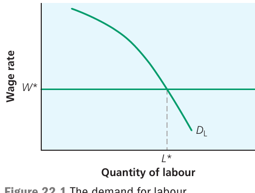
The labour demand curve slopes downward, showing an inverse relationship between wage rates and the quantity of labour firms wish to employ. At wage rate $W^*$ , firms demand $L^*$ quantity of labour.

The law of diminishing marginal productivity

An important principle underpins the downward-sloping demand curve: the law of diminishing marginal productivity. This states that as more workers are employed while other inputs (like machinery) remain constant, the additional output produced by each extra worker will eventually decline.

lightbulbExample

Worked Example: Diminishing Returns in a Kitchen

Imagine a kitchen with one oven:

Adding a second chef increases output substantially
A third chef adds some extra production
But a tenth chef, still with only one oven, adds very little additional output—chefs end up waiting around for oven space

This demonstrates how each additional worker contributes progressively less to total output when other resources remain fixed.

Since each additional worker contributes less extra output, firms will only hire more workers if the wage rate falls to match the lower additional revenue generated. This creates the downward-sloping demand relationship.

Factors affecting the position of the labour demand curve

While the demand curve shows the relationship between wages and quantity demanded, several factors can shift the entire curve's position.

Changes in labour productivity

If workers become more productive—producing more output per hour worked—then at any given wage rate, firms will want to employ more workers because each worker generates more revenue.

Productivity improvements might come from:

New technology that helps workers produce more efficiently
Better training programs
Improved management practices
Better equipment and tools

infoNote

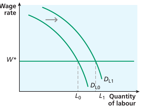
When labour productivity increases due to technological advances, the demand curve shifts rightward from $D_{L0}$ to $D_{L1}$ . At the same wage $W^*$ , firms now want to employ $L_1$ workers instead of $L_0$ .

Changes in demand for the firm's product

Since labour demand derives from the need to produce output for sale, changes in product demand directly affect labour demand.

If consumer demand for a product increases, firms can sell more output at higher prices. This makes workers more valuable because their output generates more revenue. The labour demand curve shifts to the right.

Conversely, if product demand falls—perhaps during a recession—firms need fewer workers to produce the reduced quantity of goods they can sell.

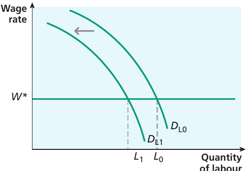
A fall in product demand causes the labour demand curve to shift leftward from $D_{L0}$ to $D_{L1}$ . At wage $W^*$ , firms now only want $L_1$ workers instead of $L_0$ , potentially leading to redundancies.

chatImportant

This explains why labour demand tends to increase during economic booms and decrease during recessions, even if worker productivity hasn't changed.

Wage elasticity of the demand for labour

Beyond understanding what shifts labour demand, we need to consider how sensitive firms are to wage changes. Wage elasticity of demand for labour measures how much the quantity of labour demanded changes in response to a wage rate change.

Several factors influence this elasticity:

Availability of substitutes

The easier it is to substitute capital equipment or other inputs for labour, the more elastic (responsive) labour demand becomes. If wages rise and firms can readily replace workers with machinery, they will do so, causing a large fall in labour quantity demanded.

lightbulbExample

Example: Automation and Substitution

Automated checkout machines can substitute for cashiers relatively easily, making labour demand more elastic in retail.

However, substituting capital for highly skilled surgeons or creative designers is much more difficult, making their labour demand more inelastic.

Whether capital can substitute for labour depends heavily on the nature of the work and available technology. Some jobs are more easily automated than others.

Share of labour in total costs

When labour represents a large proportion of a firm's total costs, demand for labour tends to be more elastic. A wage increase significantly impacts overall costs, forcing firms to respond by cutting labour use substantially.

In service industries like hairdressing or teaching, labour costs dominate. Manufacturing firms with expensive machinery may find labour is a smaller cost share, making demand less elastic.

Time period

Labour demand elasticity differs between short and long run. In the short run, capital equipment is fixed—firms cannot quickly install new machinery or reorganize production. This makes short-run labour demand relatively inelastic.

Over longer periods, firms can adjust all inputs. They might invest in labor-saving technology or restructure operations. This makes long-run labour demand more elastic—firms have more options to reduce labour use if wages rise persistently.

Price elasticity of demand for the product

There's an additional consideration unique to derived demand. If demand for the firm's product is highly price elastic, then when wage increases force up production costs and prices, sales will fall sharply. This limits how much of a wage increase firms can absorb without losing customers, making labour demand more elastic.

Labour supply

Individual labour supply

From the worker's perspective, deciding how much to work involves choosing between earning income and enjoying leisure time. Every hour worked means one less hour available for rest, hobbies, family time, or other activities.

infoNote

The wage rate represents the opportunity cost of leisure. When someone chooses an hour of leisure, they sacrifice the wages they could have earned by working that hour. Higher wages mean leisure becomes more expensive—each hour of relaxation costs more in forgone earnings.

The effect of wage rates on labour supply: two competing forces

When wages increase, workers face two contradictory effects:

chatImportant

The substitution effect: Higher wages make work more rewarding relative to leisure. Each hour of leisure now costs more in lost earnings, encouraging workers to substitute work for leisure. This effect pushes workers to supply more labour when wages rise.

The income effect: Higher wages mean workers can maintain their standard of living while working fewer hours. If leisure is a normal good (something people want more of as income rises), workers may choose to "buy" more leisure time by working less.

Which effect dominates?

At relatively low wages, the substitution effect typically outweighs the income effect. Workers are keen to earn more by working additional hours. As wages continue rising, however, the income effect may become stronger. Once workers earn enough to live comfortably, they might value extra leisure time more than additional income.

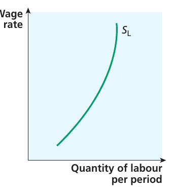
The backward-bending supply curve

This creates an interesting possibility: an individual worker's labour supply curve might bend backwards at higher wage levels.

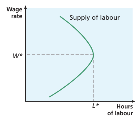
Initially, as wages rise from low levels, the worker supplies more hours (upward-sloping section). But beyond wage $W^*$ , further wage increases lead the worker to supply fewer hours (backward-bending section). The income effect has become dominant—the worker prefers more leisure to additional income.

infoNote

This isn't just theoretical. High-earning professionals sometimes reduce their working hours, choosing work-life balance over maximum income.

Non-pecuniary benefits

Workers don't make employment decisions based solely on wages. Non-pecuniary benefits—advantages that aren't monetary—can significantly influence labour supply choices.

These might include:

Job satisfaction and interesting work
Pleasant working conditions
Generous holiday allowances
Flexible working arrangements
Good pension schemes
Training and career development opportunities
Workplace facilities (gyms, cafeterias, childcare)

Firms offering attractive non-pecuniary benefits can sometimes recruit workers at lower wages than competitors. Workers effectively accept lower pay in exchange for these advantages. This can shift the position of the labour supply curve, as workers are willing to supply more labour at any given wage rate.

Industry labour supply

While individual labour supply curves might bend backwards, the labour supply curve for an entire industry or occupation typically slopes upward.

Higher wages in an industry attract workers from several sources:

Unemployed people seeking work
Workers in other industries where wages haven't risen
People not currently in the workforce (students finishing education, those taking career breaks)
Immigrants attracted by higher wages

infoNote

This gives the industry labour supply curve a conventional upward slope. Higher wages bring more workers into the industry, even if some existing workers individually choose to work fewer hours.

The participation rate

The participation rate measures the proportion of the working-age population who are either employed or actively seeking work. This excludes:

Students in full-time education
People who have taken early retirement
Those caring for children or relatives
Discouraged workers who have given up job searching

Changes affecting participation rates can shift industry labour supply:

Higher unemployment benefits might reduce participation (leftward shift)
Increased immigration expands the potential workforce (rightward shift)
Better childcare provision enables more parents to work (rightward shift)

The wage elasticity of supply

Labour supply elasticity varies across occupations and time periods.

Short-run versus long-run elasticity

In the short run, labour supply often responds sluggishly to wage changes. When wages rise in an industry, unemployed workers with the right skills might quickly fill vacancies. However, if suitable workers aren't available, supply cannot increase immediately—people need time to retrain or gain necessary qualifications.

chatImportant

This makes short-run labour supply relatively inelastic, particularly for occupations requiring extensive training. You cannot instantly create more surgeons or engineers, even if wages rise substantially.

Over longer periods, supply becomes more elastic. People can:

Complete necessary training programs
Migrate to regions where wages are higher
Shift between related occupations

Factors affecting supply elasticity

Labour supply is more elastic when:

Training requirements are minimal or short
Skills are transferable between industries
There's a large pool of suitably qualified workers
Workers are geographically mobile
Unemployment levels are high

Labour supply is more inelastic when:

Extensive education and training are required
Innate talent or ability matters (professional sports, creative fields)
Professional qualifications and licenses restrict entry
Geographic mobility is limited

Labour market equilibrium

How equilibrium is established

Market equilibrium occurs where labour demand and supply intersect. At this point, the quantity of workers firms wish to employ exactly matches the quantity workers wish to supply at the prevailing wage rate.

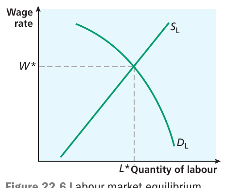
Equilibrium wage $W^*$ and employment level $L^*$ are determined where the demand curve ( $D_L$ ) intersects the supply curve ( $S_L$ ). At this wage, there are no shortages or surpluses of workers.

infoNote

If wages were below $W^*$ , firms would want to employ more workers than are available, creating a labour shortage. Firms would compete for scarce workers by offering higher wages, pushing the wage rate toward $W^*$ .

If wages were above $W^*$ , more workers would seek employment than firms wish to hire, creating unemployment. Competition among workers for scarce jobs would push wages down toward $W^*$ .

Changes in market equilibrium

Market conditions constantly change, shifting demand or supply curves and establishing new equilibrium positions.

lightbulbExample

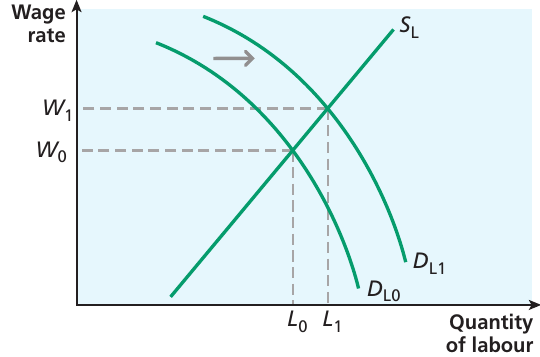
Worked Example: Market Adjustment to Increased Product Demand

Suppose demand for a product increases, shifting labour demand rightward from $D_{L0}$ to $D_{L1}$ .

Step 1: The initial equilibrium $(L_0, W_0)$ is disrupted. At the old wage $W_0$ , firms now want to employ more workers than are available. This creates a labour shortage.

Step 2: Firms respond by offering higher wages to attract workers. The wage rises to $W_1$ , and employment expands to $L_1$ . This represents the new short-run equilibrium.

Step 3: However, this might not be the end of the adjustment process. If wages in this industry have risen significantly above wages elsewhere, workers from other sectors may gradually move into this industry, shifting the labour supply curve rightward.

Long-run outcome: In a free market, this continues until wage differentials no longer provide incentives for workers to transfer between industries.

Explaining wage differentials

Why do surgeons earn vastly more than butchers? Why do professional footballers command such high salaries? Labour market analysis provides part of the answer.

Supply-side factors

Consider surgeons. The supply of surgeons is highly inelastic, particularly in the short run. Becoming a surgeon requires:

Years of demanding education and training
Significant natural ability and aptitude
Passing rigorous examinations
Gaining extensive practical experience

This creates a very limited supply. Even if surgeon wages double, the number of surgeons cannot increase quickly—it takes many years to train new ones. Moreover, not everyone has the ability to become a surgeon, regardless of the financial incentive. The limited supply, combined with relatively inelastic supply, pushes wages upward.

Butchers face quite different supply conditions. Training requirements are less demanding, and a wider range of people can acquire the necessary skills. Furthermore, butchers can transfer to other occupations in food preparation or retail if opportunities arise. This makes butcher supply more elastic—if wages fell, people would leave the trade; if wages rose substantially, more people would enter.

Demand-side factors

Supply alone doesn't determine wages—demand matters crucially too. Society places high value on skilled medical care, creating strong demand for surgeons' services. People will pay significant amounts for health treatment, generating substantial revenue that supports high surgical salaries.

infoNote

The combination of limited, inelastic supply and strong demand creates the high equilibrium wage for surgeons. Conversely, while society needs butchers, the demand doesn't generate equally high revenue, and plentiful supply keeps wages lower.

Skills, training, and barriers to entry

These examples illustrate how wage differentials reflect:

Differences in training and education requirements: Longer, more demanding training restricts supply
Natural ability and talent: Some occupations require innate abilities that only some people possess
Risk and unpleasant working conditions: Dangerous or disagreeable jobs require compensating wage differentials to attract workers
Barriers to entry: Professional licensing, union restrictions, or other barriers limit supply

Discrimination in labour markets

Wage differentials between groups don't necessarily prove discrimination exists. Different groups may have different levels of education, experience, or skills due to historical factors and educational choices made.

chatImportant

However, discrimination can contribute to wage gaps. For example, the gender pay gap—where women on average earn less than men—partly reflects:

Historical disadvantages in education and training opportunities for women
Career interruptions due to childcare responsibilities, affecting experience and seniority
Occupational segregation, with women concentrated in lower-paying sectors
Direct discrimination in hiring, promotion, or pay decisions

Policy interventions like improved childcare provision and anti-discrimination legislation aim to reduce unjustified wage differentials, though changes occur slowly as they depend on shifting social attitudes and practices built up over generations.

Market imperfections and lack of perfect competition

Labour markets often deviate from the perfectly competitive model for several reasons:

Professional regulation: Some professions strictly control entry through licensing requirements. Medical professionals, lawyers, and architects, for example, cannot practice without proper qualifications recognized by professional bodies. This restricts supply and can keep wages above competitive levels.

Trade union power: Unions may negotiate collectively on behalf of workers, potentially securing wages above the competitive equilibrium by restricting the supply of workers available to employers.

Monopsony power: In some labour markets, a single employer (or small number of employers) dominates. This gives employers market power to set wages below competitive levels.

Monopsony in a labour market

When one firm is the dominant or sole employer in a market, it faces a different situation than firms in competitive markets.

In perfect competition, firms are wage-takers—they accept the market wage and can hire as many workers as they want at that wage. The labour supply curve they face is horizontal (perfectly elastic).

A monopsonist, however, is a wage-maker. To hire more workers, it must raise the wage rate not just for new workers, but for all workers. This is because paying different wages for the same work is difficult to sustain.

infoNote

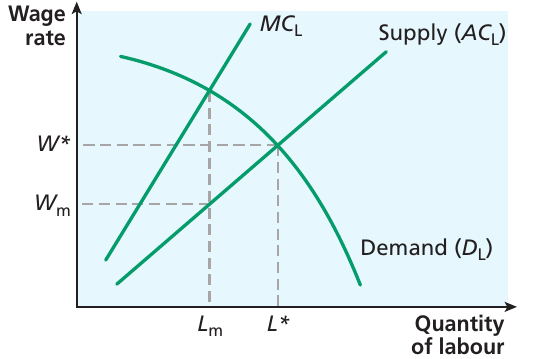
The diagram shows how monopsony differs from competition:

The supply curve ( $AC_L$ ) shows the average cost of labour—the wage rate needed to employ different quantities of workers
The marginal cost of labour ( $MC_L$ ) lies above the supply curve because hiring one more worker requires raising wages for all workers
The monopsonist maximizes profit where $MC_L$ equals labour demand ( $D_L$ ), employing $L_m$ workers
But it only needs to pay wage $W_m$ (read off the supply curve) to get workers to supply $L_m$ labour

chatImportant

Under perfect competition, equilibrium would occur at $L^*$ and $W^*$ , where demand equals supply. The monopsonist employs fewer workers ( $L_m < L^*$ ) at lower wages ( $W_m < W^*$ ).

This creates a welfare loss for society—workers who would be willing to work at wages between $W_m$ and $W^*$ , and would generate valuable output, remain unemployed because the monopsonist restricts employment to increase profits.

Examples of monopsony power include:

Single large employers dominating small towns
Specialized industries with few employers (e.g., professional sports leagues)
Public sector employers with little private sector competition (NHS in some regions)

Public sector wages

Government wages follow different determination processes than private sector wages. Rather than pure market forces, wages in the public sector result from:

Political decisions about public spending priorities
Negotiations between government and trade unions
Comparisons with private sector pay to ensure recruitment and retention
Budget constraints and taxpayer concerns about public spending

infoNote

Governments often face pressure to contain public sector wage growth to control spending. However, if public sector wages fall too far below private sector equivalents, recruitment and retention problems emerge as workers leave for better-paid private employment.

The public sector encompasses diverse occupations—from teachers and nurses to civil servants and refuse collectors—each with different supply and demand conditions. This creates complex policy challenges in setting appropriate wages across different roles while maintaining overall budget discipline.

Remember!

bookmarkSummary

Key Points to Remember:

Labour demand is derived demand: Firms want workers not for their own sake, but for the output they produce. This makes productivity and product demand crucial determinants of labour demand.
The law of diminishing marginal productivity explains why labour demand curves slope downward: as more workers are added while capital remains fixed, each additional worker contributes less extra output, so firms only hire more if wages fall.
Wage elasticity of demand depends on the substitutability between labour and capital, labour's share in total costs, the time period considered, and the price elasticity of demand for the product.
Individual labour supply involves a trade-off between income and leisure, with the wage rate representing the opportunity cost of leisure. This can create backward-bending supply curves at high wages when income effects dominate substitution effects.
Industry labour supply curves typically slope upward because higher wages attract workers from other industries, the unemployed, and outside the workforce, even though some individual workers may work fewer hours.
Labour market equilibrium occurs where supply and demand intersect, determining the wage rate and employment level. Changes in market conditions shift these curves, establishing new equilibrium positions.
Wage differentials between occupations reflect differences in supply (training requirements, natural ability, barriers to entry) and demand (revenue generated from workers' output, value society places on services).
Monopsony power allows dominant employers to pay wages below competitive levels and employ fewer workers, creating welfare losses for society.

Labour Demand, Supply, and Equilibrium (Edexcel A-Level Economics A): Revision Notes