Manipulating Worksheets (Grade 11 NSC Matric Computer Application Technology): Revision Notes
Manipulating Worksheets
Working effectively with Excel spreadsheets requires knowing how to manipulate data correctly. When you understand how to move, copy, and organise your worksheet content properly, you can avoid errors and create more professional-looking spreadsheets. This unit will teach you essential skills for working with Excel data, including how to move and copy information, control your view of the worksheet, protect your work, and prepare it for printing.
Critical Data Handling Principle
Understanding how to manipulate worksheet data is crucial because incorrect data handling can lead to broken formulas or lost information. Always ensure you're using the right method for your specific needs.
Working with sheets
When you work with Excel spreadsheets, you'll often need to reorganise your data to make it more useful or easier to read. Excel is designed to preserve important information when you move or copy cells - this means your formulas, formatting, and any comments you've added will stay intact during these operations.
Excel provides several methods for moving and copying data, each with its own advantages depending on your specific needs. The key is knowing when to use each approach for maximum effectiveness.
Why Data Preservation Matters
Excel's ability to maintain formulas, formatting, and comments during data manipulation is one of its most powerful features. This ensures that your spreadsheet's functionality remains intact even as you reorganise your information.
Moving and copying data
There are two main approaches to moving and copying data in Excel: the simple drag-and-drop method, and the more versatile cut-and-paste commands. Each method has its place in effective spreadsheet management.
Drag and drop method
The most straightforward way to move data is by using drag-and-drop. This technique works well when you're moving data within the same worksheet and can see both the source and destination locations.
Worked Example: Using Drag and Drop
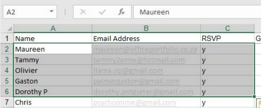
Step 1: Select the cells containing the data you want to move
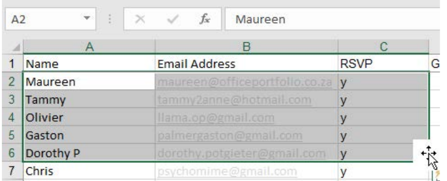
Step 2: Position your mouse cursor at the border of your selection until it changes to a move pointer (usually showing four arrows)
Step 3: Click and drag the selection to its new location
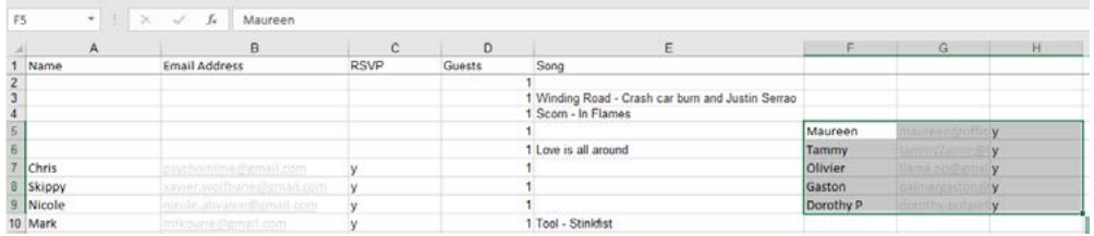
This method is particularly useful for small adjustments to your data layout, such as reordering columns in a guest list or moving a section of data to a different area of your worksheet.
Cut and paste commands
For more complex data manipulation, especially when working with large datasets or moving data between different worksheets, the Cut and Paste commands offer more control and flexibility.
The traditional Cut and Paste approach works similarly to word processing - you select your data, cut it from its original location, then paste it where you need it. This method is reliable for moving data across different parts of your workbook or even between different Excel files.
Paste special feature
Sometimes you'll need to copy only the results of formulas without copying the formulas themselves. This is where Excel's Paste Special feature becomes invaluable. This advanced tool gives you precise control over what gets copied from your source cells.
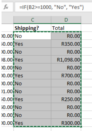
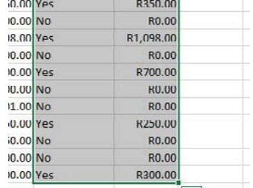
Worked Example: Using Paste Special with IF Formula
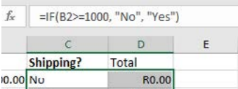
Consider a spreadsheet with an IF formula: =IF(B2>=1000,"No","Yes") that determines shipping costs.
Scenario: You want to copy just the "Yes" or "No" results to another location without copying the actual formula.
Steps:
- Select and copy your source data using the standard Copy command
- Right-click in your destination cell to open the context menu
- Select the Paste Special option from the menu
- Choose Values to paste only the results, not the formulas
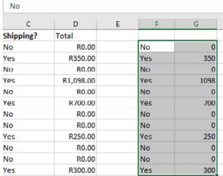
This feature is particularly useful when you're preparing data for reports or when you need to convert calculated values into static data that won't change if the original formulas are modified.
Additional Resources
Excel offers many other moving and copying options beyond these basic techniques. You can explore additional features and advanced techniques through Microsoft's support resources.
Viewing gridlines and freezing panes
When working with large spreadsheets containing many rows and columns of data, it can be challenging to keep track of which information belongs to which category. Excel provides several visual tools to help you navigate and understand your data more effectively.
Controlling gridlines
Excel displays gridlines by default to help you see the boundaries between cells. However, you can control whether these gridlines are visible, which can be useful for presentation purposes or when you want a cleaner look for your spreadsheet.
Worked Example: Controlling Gridline Display
Step 1: Navigate to the View tab in Excel's ribbon
Step 2: Look for the Gridlines option in the Show group
Step 3: Tick or untick the box to turn gridlines on or off
Freezing panes for better navigation
One of the most useful features for working with large datasets is the ability to freeze certain parts of your worksheet. This keeps important information, like column headers or row labels, visible while you scroll through the rest of your data.
Excel offers three main freezing options:
Freeze Panes: This option keeps both rows and columns visible based on your current cell selection. It's useful when you want to freeze both horizontal and vertical headers.
Freeze Top Row: This keeps the first row of your worksheet visible at all times, which is perfect for column headers.
Freeze First Column: This keeps the leftmost column visible, ideal for row labels or categories.
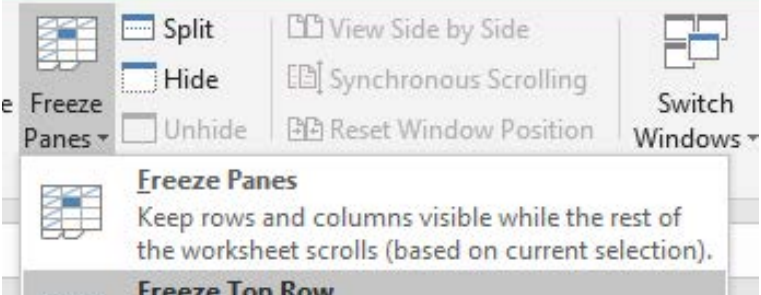
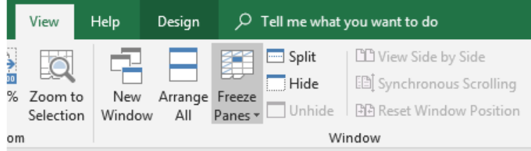
Worked Example: Freezing Panes
Step 1: Select the View tab in the Excel ribbon
Step 2: Click on Freeze Panes in the Window group
Step 3: Choose the appropriate freezing option for your needs
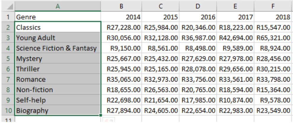
When you have a large dataset and don't want to lose track of what each column or row represents, freezing panes ensures that your headers stay in view while you scroll through your data. This is particularly helpful when working with financial data, inventory lists, or any spreadsheet where understanding the context of each cell is important.
Protecting the workbook
When you're sharing Excel workbooks with others, you may want to prevent certain types of changes to protect the integrity of your data. Excel provides comprehensive protection features that allow you to control what others can do with your spreadsheet.
Understanding worksheet protection
Worksheet protection is about preventing unauthorised changes to your spreadsheet while still allowing legitimate use. This is particularly important in business environments where multiple people might access the same file, but only certain individuals should be able to make changes.
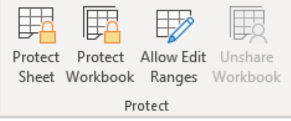
Excel's protection features include:
- Protect Sheet: Prevents changes to the current worksheet
- Protect Workbook: Prevents structural changes to the entire workbook
- Allow Edit Ranges: Permits editing of specific cell ranges only
Business Environment Considerations
In professional settings, worksheet protection is essential for maintaining data integrity when multiple users access the same spreadsheet. Always implement appropriate protection before sharing important documents.
Setting up password protection
Password protection adds a crucial layer of security to your Excel workbooks, ensuring that only authorised users can make changes to your carefully constructed spreadsheets.
Worked Example: Setting Password Protection
Step 1: Go to the Review tab in Excel's ribbon
Step 2: Click on Protect Workbook or Protect Sheet
Step 3: Enter a secure password when prompted
Step 4: Configure which actions users are allowed to perform
The protection dialogue allows you to specify exactly what users can do, such as:
- Selecting locked or unlocked cells
- Formatting cells, columns, or rows
- Inserting or deleting rows and columns
- Adding hyperlinks
Cell locking and protection
By default, all cells in Excel are set to "locked," but this locking only takes effect when you protect the worksheet. You can control which cells are locked by accessing the Format Cells dialogue.
Worked Example: Modifying Cell Protection
Step 1: Select the cells you want to modify
Step 2: Right-click and choose Format Cells
Step 3: Go to the Protection tab
Step 4: Adjust the Locked and Hidden settings as needed
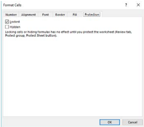
Two-Step Protection Process
Remember that locking cells or hiding formulas has no effect until you actually protect the worksheet. This two-step process gives you flexibility in setting up your protection scheme before activating it.
Print options
When you need to create hard copies of your Excel spreadsheets, understanding the available print options helps ensure your data appears exactly as you intend. Excel provides several ways to control what gets printed and how it appears on paper.
Understanding print scope
Excel gives you three main options for determining what part of your workbook gets printed:
| Print Option | Description |
|---|---|
| Print Active Sheets | Print only the sheet(s) that you have selected to print |
| Print Entire Workbook | Prints all the sheets containing data in a workbook |
| Print Selection | Prints only the cells, rows or columns you have selected |
Layout and scaling options
To make your printed spreadsheets more readable and professional, Excel offers various layout controls that help optimise your output for different purposes and paper sizes.
Professional Printing Considerations
The right combination of orientation, scaling, and margin settings can dramatically improve the readability and professional appearance of your printed spreadsheets.
Orientation control: You can switch between portrait (tall) and landscape (wide) orientation. Landscape orientation often works better for spreadsheets with many columns, as it provides more horizontal space for your data.
Scaling options: Excel can automatically adjust the size of your printed data to fit better on the page. You can:
- Print at actual size with no scaling
- Fit everything onto a single page
- Fit all columns onto one page width
- Fit all rows onto one page height
Margin adjustment: Narrower margins provide more space for your data, while wider margins can improve readability and provide space for binding.
Page break control: You can manually control where pages break when printing, ensuring that related information stays together.
These printing features help ensure that your spreadsheet data translates effectively from screen to paper, maintaining clarity and professionalism in your printed documents.
Key Points to Remember:
- Moving data preserves everything: When you move or copy cells in Excel, formulas, formatting, and comments stay intact
- Drag-and-drop for simple moves: Use drag-and-drop when moving data short distances within the same worksheet
- Paste Special for values only: Use Paste Special when you need to copy results without copying the underlying formulas
- Freeze panes for navigation: Keep headers visible by freezing the top row, first column, or custom selections when working with large datasets
- Protect before sharing: Always set up appropriate worksheet protection and passwords before sharing important spreadsheets with others