General Normal Distributions (HSC SSCE Mathematics Advanced): Revision Notes
General Normal Distributions
Introduction to general normal distributions
When we examine real-world data, we often find that it follows a bell-shaped curve pattern. For instance, when tossing 20 coins repeatedly and counting the number of heads, the resulting distribution looks very much like a normal curve. However, this curve differs from the standard normal distribution in two important ways: the mean is not zero, and the standard deviation is not equal to 1.
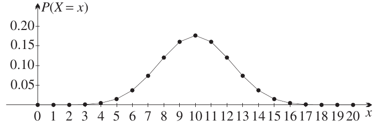
The distribution shown above is centred at (not 0) and has a spread that's wider than the standard normal distribution. This tells us we need a way to work with normal distributions that have any mean and any standard deviation, not just the standard normal with and .
A general normal distribution is a bell-shaped probability distribution that can be centred anywhere on the number line and can have any degree of spread. We create these distributions by transforming the standard normal distribution through stretching and shifting operations.
Transforming the standard normal distribution
To create a general normal distribution with mean and standard deviation , we apply a sequence of transformations to the standard normal distribution. Think of this as reshaping and repositioning the standard bell curve to match our data.
Stretching to accommodate the standard deviation
The first transformation adjusts the spread of the distribution to match the desired standard deviation .
Step 1: Horizontal stretching
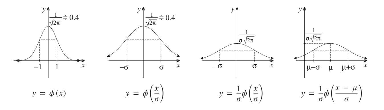
We begin by stretching the standard normal curve horizontally by a factor of . This is achieved mathematically by replacing with in the standard normal formula.
The standard normal PDF is:
After horizontal stretching, this becomes:
This stretching has an important consequence: the inflection points (the points where the curve changes from concave down to concave up) move from to .
Step 2: Vertical adjustment
However, horizontal stretching increases the area under the curve by a factor of . Since we need the total area to remain 1 (the total probability must equal 1), we must compress the curve vertically by multiplying by :
Now we have a proper probability density function with area 1, spread controlled by , but still centred at 0.
Shifting to accommodate the mean
The final transformation moves the entire curve horizontally to centre it at the desired mean .
Horizontal translation
We shift the curve units to the right by replacing with :
This translation doesn't change the area under the curve or the positions of the inflection points relative to the centre. The inflection points are now located at and , exactly one standard deviation on either side of the mean.
The general normal distribution formula
Complete formula
Let be the probability density function for a general normal distribution with mean and standard deviation . The transformation process gives us:
Alternatively, writing out the exponential form in full:
Key properties
For a general normal distribution with mean and standard deviation :
- The curve is bell-shaped and symmetric about the vertical line
- The total area under the curve equals 1 (it's a valid probability density function)
- The mean, median, and mode all coincide at
- The points of inflection occur at and (one standard deviation from the mean)
- The curve approaches but never touches the horizontal axis as
Connection to the standard normal
The general normal distribution is simply a transformed version of the standard normal. This relationship is captured in the formula:
This means we can use everything we know about the standard normal distribution to work with any normal distribution, as long as we make appropriate conversions using and .
Comparing with real data
Let's return to our coin-tossing example. When we toss 20 fair coins repeatedly and count the heads, the mean number of heads is 10 and the standard deviation is . We can overlay a normal distribution with and on our experimental data:
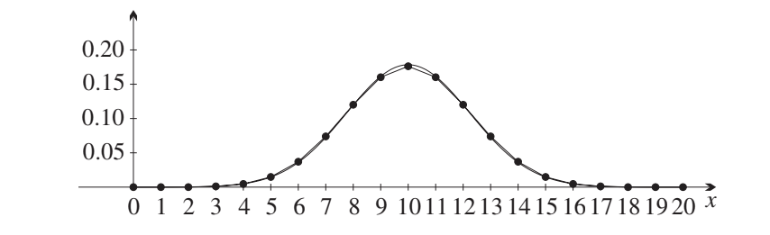
The fit is remarkably good, though not perfect. This demonstrates how the normal distribution can approximate complex real-world probability distributions. As we increase the number of coin tosses, the fit becomes even better. This historical example was actually one of the first uses of the normal distribution to approximate another probability distribution.
Working with z-scores
What is a z-score?
When working with general normal distributions, we need a way to standardise values so we can use standard normal distribution tables and results. This is where z-scores come in.
The z-score of a value tells us how many standard deviations that value lies above or below the mean. If the z-score is positive, is above the mean; if negative, is below the mean.
Conversion formulas
There are two essential formulas for converting between raw scores ( values) and z-scores:
From raw score to z-score:
From z-score to raw score:
For sample data (rather than population data), we use the sample mean and sample standard deviation instead:
Example conversion table
Here's how z-scores correspond to raw scores for a distribution with mean and standard deviation :
| 4 | 5 | 6 | 7 | 8 | 9 | 10 | 11 | 12 | 13 | 14 | 15 | 16 | |
|---|---|---|---|---|---|---|---|---|---|---|---|---|---|
| -3 | -2.5 | -2 | -1.5 | -1 | -0.5 | 0 | 0.5 | 1 | 1.5 | 2 | 2.5 | 3 |
Notice how the mean () corresponds to , and values that are 1, 2, or 3 standard deviations away from the mean have z-scores of , , or respectively.
Worked examples with z-scores
Worked Example: Converting between scores and z-scores
A dataset has mean and standard deviation .
(a) What scores would be 1, 2, and 3 standard deviations from the mean?
(b) How many standard deviations from the mean are scores of 24, 11, and 7.7?
Solution:
(a) We need to find the raw scores that correspond to , , and .
Using the formula :
- For :
- For :
- For :
- For :
- For :
- For :
(b) We need to calculate z-scores using the formula :
For :
This score is 3.33 standard deviations above the mean.
For :
This score is 0.28 standard deviations below the mean.
For :
This score is 1.19 standard deviations below the mean.
Using z-scores for probability calculations
Worked Example: Z-scores and probability
A normally distributed random variable has mean 100 and standard deviation 20.
(a) Write down the conversion formulas.
(b) Find: (i) (ii)
(c) Find the value of such that .
Solution:
(a) The conversion formulas are:
(b)(i) For :
Therefore, (from standard normal table)
(b)(ii) For :
Therefore, (using symmetry)
(c) From the standard normal table, we need to find such that .
Looking at the table: and
By interpolation:
Converting back to :
The empirical rule for general normal distributions
The 68-95-99.7 rule
One of the most useful properties of the normal distribution is the empirical rule, also called the 68-95-99.7 rule. When a random variable follows a normal distribution with mean and standard deviation :
- Approximately 68% of values lie within one standard deviation of the mean:
- Approximately 95% of values lie within two standard deviations of the mean:
- Approximately 99.7% of values lie within three standard deviations of the mean:
This rule is incredibly useful for quick mental calculations and for understanding what values are typical or unusual in a dataset.
Quartiles for normal distributions
The quartiles divide the distribution into quarters. For any normal distribution:
First quartile (Q₁): The value below which 25% of the data falls
Second quartile (Q₂): The median, which equals the mean for normal distributions
Third quartile (Q₃): The value below which 75% of the data falls
Interquartile range (IQR): The range of the middle 50% of the data
The IQR criterion for outliers
The IQR criterion is a common method for identifying outliers in a dataset. A value is considered an outlier if it lies outside the range:
For a normal distribution, this translates to:
Any value outside this interval is flagged as a potential outlier. For a normal distribution, approximately 0.7% of values (about 7 in 1000) will be classified as outliers using this criterion.
Applying the empirical rule in practice
Worked Example: Applying the empirical rule
A dataset with 1000 scores is known to be sampled from a normally distributed variable with mean and standard deviation .
(a) Describe what the empirical rule predicts about the data.
(b) Predict roughly how many scores will: (i) lie in , (ii) lie in , (iii) lie in .
(c) Using the IQR criterion, roughly how many outliers would you expect?
Solution:
(a) Applying the empirical rule:
Within 1 SD:
About scores will fall in this range.
Within 2 SDs:
About scores will fall in this range.
Within 3 SDs:
About scores will fall in this range.
(b)(i) For :
Predicted number of scores: scores
(b)(ii) For :
Predicted number of scores: scores
(b)(iii) For the interval :
Predicted number of scores: scores
(c) The IQR criterion identifies values outside to as outliers.
For any normal distribution, approximately 7 in 1000 scores (0.7%) are classified as outliers by this criterion.
Therefore, we expect about 7 outliers in this dataset.
Key takeaways
Key Points to Remember:
-
Any normal distribution can be created by stretching and shifting the standard normal distribution.
-
The general normal PDF is: or equivalently
-
Z-scores allow us to standardise any normal distribution: and
-
The empirical rule (68-95-99.7) tells us that approximately 68%, 95%, and 99.7% of values lie within 1, 2, and 3 standard deviations of the mean respectively.
-
For a normal distribution: , , and
-
The IQR criterion identifies outliers as values outside to