The Standard Normal Distribution (HSC SSCE Mathematics Advanced): Revision Notes
The Standard Normal Distribution
Introduction to the standard normal distribution
The standard normal distribution is a special type of continuous probability distribution that plays a central role in statistics. It belongs to a family of distributions called Gaussian or normal distributions, which are characterised by their distinctive bell-shaped curves.
The standard normal distribution is particularly important because:
- It occurs naturally in many real-world situations
- Every normal distribution can be transformed into the standard normal distribution
- It serves as a reference distribution for statistical analysis
The random variable for the standard normal distribution is denoted by (rather than ), and its values are written as (rather than ).
The probability density function
The probability density function (PDF) of the standard normal distribution is denoted by , where is the Greek letter phi (corresponding to Latin f).
The formula for the PDF is:
Practical approximation: The constant , so we can think of the formula approximately as:
This makes the formula easier to work with mentally.
Properties of the bell curve
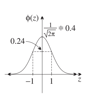
The graph of has several important characteristics:
Shape and symmetry:
- The y-intercept is (because )
- The maximum value occurs at , making this the mode
- The function is even, meaning it has line symmetry about the y-axis
- Replacing with leaves the equation unchanged:
Domain and range:
- The function is defined for all real values of
- The function is always positive: for all
Asymptotic behaviour:
- As or , the function approaches zero
- The z-axis acts as a horizontal asymptote in both directions
Inflection points:
- The curve has points of inflection at and
- At these points, the y-coordinate is
Mean and variance
The standard normal distribution has two defining parameters:
- Mean:
- Variance:
- Standard deviation:
These values are reflected in the graph:
- The mean corresponds to the centre of symmetry and the maximum turning point
- The inflection points at and are each one standard deviation from the mean
Practical tip: When you see any bell-shaped curve, first identify the turning point (the mean), then locate the inflection points (one standard deviation away from the mean on each side).
The cumulative distribution function
While the PDF tells us the probability density at each point, to calculate actual probabilities we need the cumulative distribution function (CDF), denoted by (uppercase phi).
The CDF is defined as:
This represents the probability that , which equals the area under the PDF curve from to .
Important properties of the CDF:
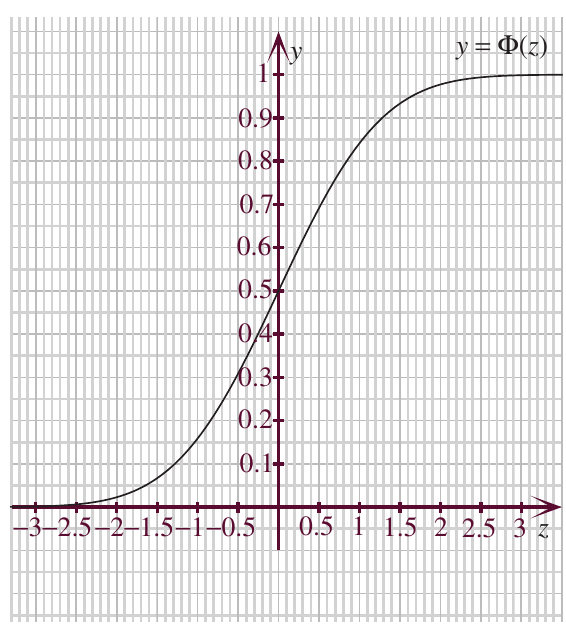
- The graph of is S-shaped (sigmoid)
- It has horizontal asymptotes: on the left and on the right
- It has point symmetry about the point
- At , exactly half the area lies to the left:
Using z-tables to find probabilities
The integral defining cannot be calculated using standard calculus techniques. Instead, we use:
- z-tables (statistical tables showing values of )
- Statistical calculators with built-in functions
- Spreadsheet functions (e.g., Excel's NORM.S.DIST function)
- Statistical software
Reading the z-table
Here is a standard z-table showing values of for positive z-values:
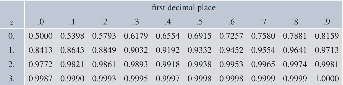
How to read the table:
- Find the first decimal place of in the left column
- Find the second decimal place in the top row
- The intersection gives
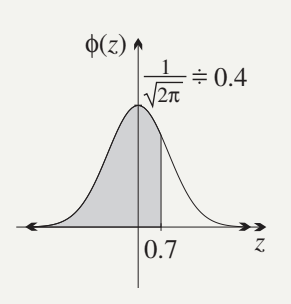
Reading the z-table: Finding
To find :
- Look at row starting with "0."
- Move to column headed ".7"
- Read the value:
The table only shows positive z-values because we can use symmetry to find negative values.
Calculating probabilities
To find probabilities for the standard normal distribution, we combine the CDF values with two key principles:
Key Principles:
- The total area under the curve equals 1
- The curve is symmetric about the y-axis
Basic probability calculations
Right-tail probability:
This works because the total area is 1, so the area to the right equals 1 minus the area to the left.
Left-tail probability:
This uses the symmetry property: the area to the left of equals the area to the right of .
Central probability from zero:
This subtracts the left-half area from the total area up to .
Central probability symmetric about zero:
Alternatively, using symmetry:
Important note: For continuous distributions, , so there's no need to distinguish between and , or between and .
Worked example: Finding probabilities
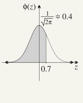
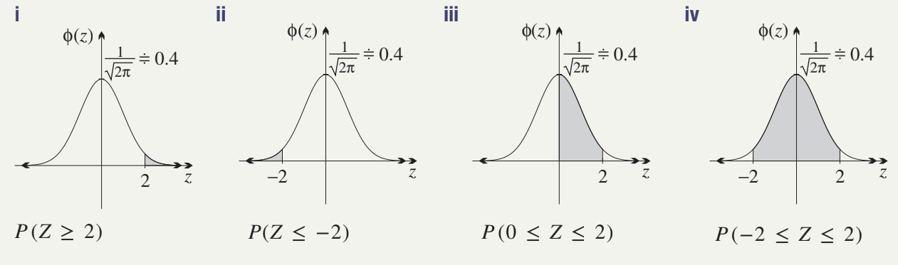
Worked Example: Finding Various Probabilities
Let's find various probabilities when .
a) Finding :
From the z-table:
b) i) Finding :
Using the complement:
b) ii) Finding :
Using symmetry:
b) iii) Finding :
Subtracting areas:
b) iv) Finding :
Method 1: Using subtraction:
Method 2: Using symmetry:
Working with negative z-values
When dealing with negative z-values, always use the symmetry of the normal curve.
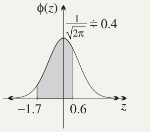
Worked Example: Finding
Using symmetry, this equals :
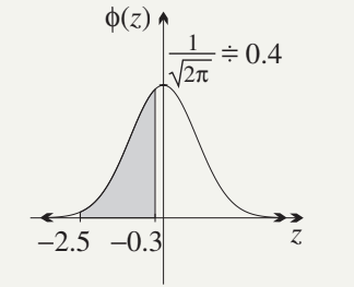
Worked Example: Finding
Split the interval at zero:
Using symmetry on the first part:
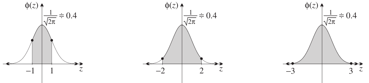
The empirical rule (68-95-99.7 rule)
A particularly useful approximation for normal distributions is the empirical rule, which tells us what proportion of data falls within 1, 2, or 3 standard deviations of the mean.
For the standard normal distribution, where :
- Approximately 68% of values fall within :
- Approximately 95% of values fall within :
- Approximately 99.7% of values fall within :
Why is this useful?
The empirical rule provides quick mental estimates without needing tables or calculators. It's particularly helpful for:
- Checking if calculations are reasonable
- Making quick probability estimates
- Understanding what "typical" values look like in a normal distribution
Using the empirical rule in practice
Worked Example: Using the Empirical Rule
An experiment is run 1000 times with a standard normal random variable .
a) How many scores greater than 2 would you expect?
By the empirical rule:
- We expect scores within
- By symmetry, half of these (475 scores) fall within
- Since 500 scores should be positive, we expect scores greater than 2
We expect approximately 25 scores greater than 2
b) Find if we expect about 840 scores greater than :
- We expect 160 scores less than , so must be negative
- By symmetry, we also expect 160 scores greater than
- Therefore: scores fall between and
- This represents 68% of scores, so by the empirical rule:
Quartiles and percentiles
Quartiles and percentiles can be found from the graph of the CDF or by using interpolation on z-tables.
Key values for the standard normal distribution
Quartiles:
- First quartile:
- Second quartile (median): (by symmetry)
- Third quartile:
Interquartile range: IQR
Finding quartiles and percentiles
Worked Example: Finding the 9th Decile
Find the 9th decile (90th percentile) of the standard normal distribution.
We need to solve
From the z-table:
Using interpolation, the 9th decile is approximately
Worked Example: Finding the Third Quartile
Find the third quartile .
We need to solve
From the z-table:
Using interpolation:
By symmetry:
Therefore: IQR
The IQR criterion for outliers
Using the IQR criterion, an outlier is any value outside:
For the standard normal distribution:
So an outlier lies outside
The probability of being an outlier:
This means approximately 7 in 1000 scores (or just under 1%) would be classified as outliers.
Summary
Key Points to Remember:
-
The standard normal distribution has PDF with mean and standard deviation
-
The bell-shaped curve is symmetric about with maximum at and inflection points at
-
Use the CDF and z-tables to calculate probabilities, applying symmetry for negative z-values
-
The empirical rule states that approximately 68%, 95%, and 99.7% of data falls within 1, 2, and 3 standard deviations of the mean respectively
-
For continuous distributions, , so strict and non-strict inequalities give the same probability