A Curve-Sketching Menu Revision Notes for HSC SSCE Mathematics Advanced

A Curve-Sketching Menu

Understanding curve sketching

When working with unfamiliar functions, you need a reliable approach to understand their behaviour and produce accurate sketches. A sketch is different from a precise plot - it's a clear diagram that captures the essential features of a curve without requiring exact plotting of every point.

infoNote

A "sketch" of a graph is not an accurate plot. It is a neat diagram showing the main features of the curve - the big picture of how the function behaves.

The curve-sketching menu presented here brings together four key techniques into a systematic process. This method works well for many common functions, though it cannot handle every possible case. As you progress in your studies, additional techniques involving calculus will expand what you can analyse.

What makes a good sketch

A proper mathematical sketch must include certain key features to be useful. The goal is to communicate the function's behaviour clearly through a well-organized diagram.

chatImportant

Essential elements of any sketch:

All x-intercepts and y-intercepts (when they can be found)
Any vertical asymptotes
Any horizontal asymptotes
Other significant points on the curve
Labels on both axes
Some indication of scale on both axes

Remember that a sketch shows the general shape and important features, not every tiny detail.

The curve-sketching menu

Here is a systematic approach for sketching an unknown function. Follow these steps in order to build up a complete picture of the function's behaviour.

Step 0 - Preparation

Before analyzing the function, simplify it as much as possible. Combine any fractions using a common denominator, then factorise both the numerator and denominator completely. This preparation makes the remaining steps much easier.

infoNote

Think of Step 0 as "cleaning up" the function. A well-prepared function reveals its key features much more readily in the steps that follow.

Step 1 - Domain

Always start by finding the domain. Ask yourself: what values of $x$ are allowed? Look for values where the function is undefined (such as where a denominator equals zero). The domain tells you where the function exists.

chatImportant

Finding the domain first is crucial - it reveals any discontinuities that might lead to vertical asymptotes and prevents you from trying to evaluate the function at impossible values.

Step 2 - Symmetry

Check whether the function has any symmetry:

If $f(-x) = f(x)$ , the function is even and has line symmetry in the y-axis
If $f(-x) = -f(x)$ , the function is odd and has point symmetry about the origin
Otherwise, the function has neither type of symmetry

Identifying symmetry can save you work and helps you understand the function's shape.

Step 3A - Intercepts

Find where the curve crosses the axes:

y-intercept: Substitute $x = 0$ into the function
x-intercepts (zeroes): Solve $f(x) = 0$ to find where the curve crosses the x-axis

Step 3B - Sign

Determine where the function is positive and where it is negative. Use a table of test values, checking the sign of $f(x)$ in each region between zeroes and discontinuities. This tells you which parts of the curve lie above or below the x-axis.

Step 4A - Vertical asymptotes

Examine the behaviour near any discontinuities. A vertical asymptote occurs at $x = a$ when the denominator equals zero but the numerator does not. Investigate what happens as $x$ approaches the discontinuity from each side.

Step 4B - Horizontal asymptotes

Examine what happens as $x \to \infty$ and as $x \to -\infty$ . If the function approaches a constant value $L$ , then $y = L$ is a horizontal asymptote.

Worked example 1: even rational function

lightbulbExample

Worked Example: Sketching an Even Rational Function

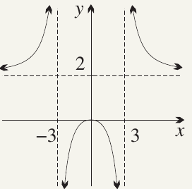
Question: Sketch $f(x) = \dfrac{2x^2}{x^2 - 9}$

Solution:

Step 0 - Preparation:

Factorise the denominator: $f(x) = \dfrac{2x^2}{(x-3)(x+3)}$

Step 1 - Domain:

The function is undefined where the denominator equals zero.

Setting $(x-3)(x+3) = 0$ gives $x = 3$ or $x = -3$

Domain: $x \neq 3$ and $x \neq -3$

Step 2 - Symmetry:

Test if the function is even: $f(-x) = \dfrac{2(-x)^2}{(-x)^2 - 9}$

$f(-x) = \dfrac{2x^2}{x^2 - 9}$

$f(-x) = f(x)$

Since $f(-x) = f(x)$ , the function is even and has line symmetry in the y-axis.

Step 3 - Intercepts and sign:

When $x = 0$ : $y = \dfrac{2(0)^2}{0^2 - 9} = 0$

The function has a zero at $x = 0$ and discontinuities at $x = 3$ and $x = -3$ .

Testing values in each region:

$x$	$-4$	$-3$	$-1$	$0$	$1$	$3$	$4$
$f(x)$	$\dfrac{32}{7}$	*	$-\dfrac{1}{4}$	$0$	$-\dfrac{1}{4}$	*	$\dfrac{32}{7}$
sign	$+$	*	$-$	$0$	$-$	*	$+$

The asterisks (*) indicate discontinuities.

Step 4A - Vertical asymptotes:

At $x = 3$ and $x = -3$ , the denominator equals zero but the numerator does not, so these are vertical asymptotes.

From the sign table:

$f(x) \to \infty$ as $x \to 3^+$ and $f(x) \to -\infty$ as $x \to 3^-$
$f(x) \to -\infty$ as $x \to (-3)^+$ and $f(x) \to \infty$ as $x \to (-3)^-$

Step 4B - Horizontal asymptotes:

Divide numerator and denominator by $x^2$ : $f(x) = \dfrac{2}{1 - \dfrac{9}{x^2}}$

As $x \to \infty$ , $\dfrac{9}{x^2} \to 0$

Therefore $f(x) \to 2$ as $x \to \infty$ and as $x \to -\infty$

The line $y = 2$ is a horizontal asymptote.

Worked example 2: sum of fractions

lightbulbExample

Worked Example: Sketching a Sum of Fractions

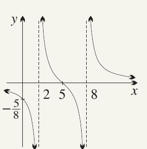
Question: Sketch $f(x) = \dfrac{1}{x-2} + \dfrac{1}{x-8}$

Solution:

Step 0 - Preparation:

Find a common denominator: $f(x) = \dfrac{(x-8) + (x-2)}{(x-2)(x-8)}$

$f(x) = \dfrac{2x - 10}{(x-2)(x-8)}$

Factorise the numerator: $f(x) = \dfrac{2(x-5)}{(x-2)(x-8)}$

Step 1 - Domain:

The domain is $x \neq 2$ and $x \neq 8$

Step 2 - Symmetry:

Testing shows that $f(x)$ is neither even nor odd.

Step 3 - Intercepts and sign:

When $x = 0$ : $y = \dfrac{2(0-5)}{(0-2)(0-8)} = \dfrac{-10}{16} = -\dfrac{5}{8}$

The y-intercept is at $\left(0, -\dfrac{5}{8}\right)$

There is a zero at $x = 5$ (where the numerator equals zero) and discontinuities at $x = 2$ and $x = 8$ .

Using a sign analysis table:

$x$	$0$	$2$	$3$	$5$	$7$	$8$	$10$
$x-2$	$-$	$0$	$+$	$+$	$+$	$+$	$+$
$x-5$	$-$	$-$	$-$	$0$	$+$	$+$	$+$
$x-8$	$-$	$-$	$-$	$-$	$-$	$0$	$+$
$f(x)$	$-$	*	$+$	$0$	$-$	*	$+$

The asterisks indicate discontinuities. This table shows that:

$f(x) < 0$ when $x < 2$
$f(x) > 0$ when $2 < x < 5$
$f(x) < 0$ when $5 < x < 8$
$f(x) > 0$ when $x > 8$

Step 4 - Asymptotes:

At $x = 2$ and $x = 8$ , the denominator equals zero but the numerator does not, so $x = 2$ and $x = 8$ are vertical asymptotes.

For horizontal asymptotes, look at the original form of the function:

As $x \to \infty$ : both $\dfrac{1}{x-2} \to 0$ and $\dfrac{1}{x-8} \to 0$

Therefore $f(x) \to 0$ as $x \to \infty$ and as $x \to -\infty$

The line $y = 0$ (the x-axis) is a horizontal asymptote.

Remember!

bookmarkSummary

Key Points to Remember:

A sketch is not a plot: Show the key features clearly with labeled axes and scale, but don't worry about plotting every point precisely
Always find the domain first: This tells you where the function exists and reveals any discontinuities that might lead to vertical asymptotes
Check for symmetry early: If a function is even or odd, you only need to sketch half of it and use symmetry for the rest
Vertical asymptotes occur where denominators vanish: Look for values where the denominator equals zero but the numerator doesn't - these create vertical asymptotes
Sign analysis is crucial: A table showing where the function is positive or negative helps you understand which parts of the curve sit above or below the x-axis

A Curve-Sketching Menu (HSC SSCE Mathematics Advanced): Revision Notes