Rates and Integration (HSC SSCE Mathematics Advanced): Revision Notes

Worked Example: Tank Drainage Problem

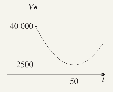
Problem: A tank contains 40,000 litres of water. When the draining valve is opened, the volume $V$ in litres decreases at a variable rate given by $\frac{dV}{dt} = -1500 + 30t$, where $t$ is the time in seconds after opening the valve. The valve shuts off once water stops flowing.

Part a: When does the water stop flowing?

Water stops flowing when the rate becomes zero. Setting the rate equal to zero:

$\frac{dV}{dt} = 0$

$-1500 + 30t = 0$

$30t = 1500$

$t = 50$

The water stops flowing after 50 seconds.

Part b: Why is the rate negative?

During the first 50 seconds, water is flowing out of the tank. This means the volume $V$ in the tank is decreasing. When a quantity decreases over time, its rate of change (derivative) is negative. This is why $\frac{dV}{dt}$ is negative up to $t = 50$ seconds.

Part c: Finding the volume function

To find the volume at any time, we integrate the rate:

$V = \int (-1500 + 30t) \, dt$

$V = -1500t + 15t^2 + C$

Now we use the initial condition to find $C$. We're told that when $t = 0$, the tank contains $V = 40,000$ litres.

Substituting these values:

$40,000 = -1500(0) + 15(0)^2 + C$

$40,000 = 0 + 0 + C$

$C = 40,000$

Therefore, the volume at any time $t$ is:

$V = 40,000 - 1500t + 15t^2$

The graph shows how the volume decreases from 40,000 litres, reaches a minimum of 2,500 litres at $t = 50$ seconds, then the dashed line indicates the valve has shut off.

Part d: How much water has flowed out?

When $t = 50$ seconds:

$V = 40,000 - 1500(50) + 15(2500)$

$V = 40,000 - 75,000 + 37,500$

$V = 2,500 \text{ litres}$

The tank still contains 2,500 litres when the valve closes. Since it started with 40,000 litres:

Amount that flowed out $= 40,000 - 2,500 = 37,500$ litres

Answer: 37,500 litres of water flowed out

Worked Example: Analyzing Population from Rate Graph

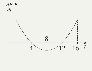
Problem: Frog numbers in the Ranavilla district were increasing, but during a drought, the rate of increase fell and became negative for several years. The graph below shows the rate $\frac{dP}{dt}$ of population growth as a function of time $t$ years after observations began.

Part a: When was the population neither increasing nor decreasing?

Looking at the graph, $\frac{dP}{dt} = 0$ at two times:

• When $t = 4$ years
• When $t = 12$ years

These are the times when the population was stationary (neither increasing nor decreasing).

Part b: When was the population decreasing and increasing?

The population decreases when its rate of change is negative. From the graph:

• $\frac{dP}{dt} < 0$ (negative) when $4 < t < 12$
• Therefore, the population was decreasing during years 4 to 12

The population increases when its rate of change is positive. From the graph:

• $\frac{dP}{dt} > 0$ (positive) when $0 < t < 4$ and when $12 < t < 16$
• Therefore, the population was increasing during years 0 to 4, and again during years 12 to 16

Part c: When was the population decreasing most rapidly?

The population decreases most rapidly when the rate $\frac{dP}{dt}$ is at its most negative value (the minimum point on the graph). This occurs at t = 8 years.

Part d: When was the population at a maximum?

From parts a and b, we know that:

• Before $t = 4$, the population was increasing
• After $t = 4$, the population was decreasing

Therefore, the population reached its maximum at t = 4 years.

Part e: When was the population at a minimum?

Similarly, we can see that:

• Before $t = 12$, the population was decreasing
• After $t = 12$, the population was increasing

Therefore, the population reached its minimum at t = 12 years.

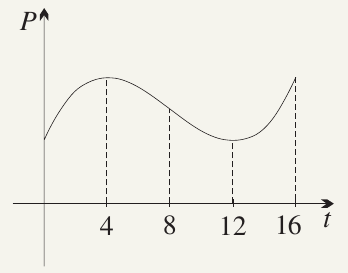
Part f: Sketching the population graph

We need to draw a graph of $P$ versus $t$ that matches the behaviour we identified. The key features are:

• The gradient of $P$ must match the values shown in the $\frac{dP}{dt}$ graph
• Maximum at $t = 4$ years
• Minimum at $t = 12$ years
• Increasing before $t = 4$ and after $t = 12$
• Decreasing between $t = 4$ and $t = 12$
• The population cannot fall below zero

Worked Example: Water Flow with Exponential Decay

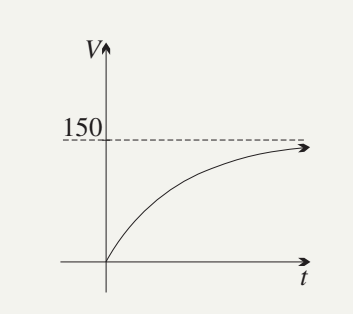
Problem: During a drought, the flow rate of water from Welcome Well gradually diminishes according to $\frac{dV}{dt} = 3e^{-0.02t}$, where $V$ is the volume in megalitres that has flowed out during the first $t$ days after time zero.

Part a: Is the rate always positive?

Since $e^x > 0$ for all values of $x$, we know that $e^{-0.02t} > 0$ for all values of $t$.

Therefore, $\frac{dV}{dt} = 3e^{-0.02t}$ is always positive.

Physical significance: The volume $V$ represents the total amount of water that has flowed out of the well. This quantity can only increase (water flows out, not back in), so its rate of change must always be positive. The water continues to flow, just at an ever-decreasing rate.

Part b: Finding the volume function

Integrating the rate:

$V = \int 3e^{-0.02t} \, dt$

$V = -150e^{-0.02t} + C$

When $t = 0$, no water has yet flowed out, so $V = 0$.

Substituting:

$0 = -150e^{0} + C$

$0 = -150(1) + C$

$C = 150$

Therefore:

$V = -150e^{-0.02t} + 150$

$V = 150(1 - e^{-0.02t})$

Part c: Water flow during first 100 days

When $t = 100$ days:

$V = 150(1 - e^{-2})$

$V \approx 129.7 \text{ megalitres}$

Part d: Long-term behaviour and percentage analysis

As $t \to \infty$, the exponential term $e^{-0.02t} \to 0$

Therefore, $V \to 150$ megalitres

This means the well will eventually produce a total of 150 megalitres of water, but it approaches this limit asymptotically (never quite reaching it in finite time).

To find what percentage flows in the first 100 days:

$\text{Percentage} = \frac{\text{Flow in first 100 days}}{\text{Total flow}} \times 100\%$

$= \frac{150(1 - e^{-2})}{150} \times 100\%$

$= (1 - e^{-2}) \times 100\%$

$= 0.86466... \times 100\%$

$\approx 86.5\%$

Answer: Approximately 86.5% of the total water flow occurs in the first 100 days, even though water continues to flow indefinitely at an ever-decreasing rate.