Velocity and Acceleration as Derivatives (HSC SSCE Mathematics Advanced): Revision Notes

Worked Example: Ball Trajectory Analysis

A ball moves with displacement equation $x = 5t(8 - t)$, where $x$ is in metres and $t$ is in seconds.

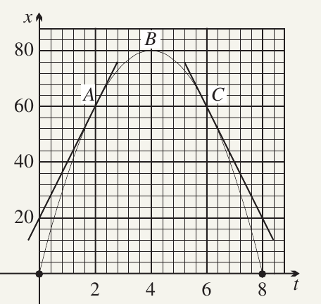
Step 1: Finding the velocity function

First, expand the displacement equation:

$x = 5t(8 - t)$

$x = 40t - 5t^2$

Differentiate to find velocity:

$v = \frac{dx}{dt} = 40 - 10t$

This is a linear function with $v$-intercept 40 and gradient $-10$.

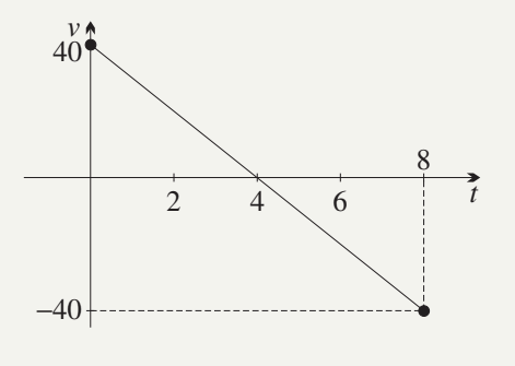
Step 2: Creating a table of values

The velocity graph is a straight line sloping downward.

Step 3: Checking against tangent gradients

If you measure the gradients of the tangents at points A ($t = 2$), B ($t = 4$), and C ($t = 6$) on the displacement graph, they match the velocity values: 20, 0, and -20 respectively.

Step 4: Determining initial velocity

When $t = 0$, $v = 40$

The ball was originally hit upwards at 40 m/s.

Step 5: Finding impact speed

When $t = 8$, $v = -40$

The ball hits the ground at 40 m/s (the negative sign indicates downward direction).

Worked Example: Cubic Motion Analysis

A particle moves with displacement $x = t^3 - 6t - 2$ (in metres and seconds).

Step 1: Finding velocity

$x = t^3 - 6t - 2$

$v = \frac{dx}{dt} = 3t^2 - 6$

Step 2: Analysis at $t = 0$

$x = -2 \text{ (displacement is -2 metres)}$

$v = -6 \text{ (velocity is -6 m/s)}$

Distance from origin: 2 metres

Speed: 6 m/s

Step 3: Analysis at $t = 3$

$x = 27 - 18 - 2 = 7 \text{ (displacement is 7 metres)}$

$v = 27 - 6 = 21 \text{ (velocity is 21 m/s)}$

Distance from origin: 7 metres

Speed: 21 m/s

Worked Example: Finding When a Particle is Stationary

A particle moves with displacement $x = \frac{1}{3}t^3 - 6t^2 + 27t - 18$ (in metres and seconds).

Step 1: Finding when stationary

First, find the velocity function:

$x = \frac{1}{3}t^3 - 6t^2 + 27t - 18$

$v = \frac{dx}{dt} = t^2 - 12t + 27$

Factor the quadratic:

$v = (t - 3)(t - 9)$

Set $v = 0$:

$(t - 3)(t - 9) = 0$

$t = 3 \text{ or } t = 9$

The particle is stationary after 3 seconds and after 9 seconds.

Step 2: Finding distance from origin

When $t = 3$:

$x = 9 - 54 + 81 - 18 = 18 \text{ metres}$

When $t = 9$:

$x = 243 - 486 + 243 - 18 = -18 \text{ metres}$

The particle is 18 metres from the origin on both occasions (once at +18, once at -18).

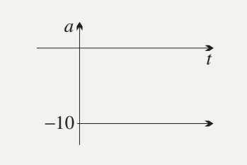
Worked Example: Constant Acceleration Analysis

Consider the ball from earlier with displacement $x = 5t(8 - t)$.

Step 1: Finding velocity and acceleration

$x = 40t - 5t^2$

$v = \frac{dx}{dt} = 40 - 10t$

$a = \frac{dv}{dt} = -10$

The acceleration is constant at -10 m/s².

Step 2: Analysis at $t = 2$

$x = 60 \text{ (displacement is 60 metres above ground)}$

$v = 20 \text{ (velocity is 20 m/s upwards)}$

$a = -10 \text{ (acceleration is 10 m/s² downwards)}$

Step 3: Understanding the motion

During the first 4 seconds:

• The ball has positive velocity (rising)
• The ball is slowing down by 10 m/s every second

During the last 4 seconds:

• The ball has negative velocity (falling)
• The ball is speeding up by 10 m/s every second

This shows how constant negative acceleration can cause a particle to both slow down (when moving upward) and speed up (when moving downward).

Worked Example: Finding When Acceleration is Zero

For the particle with displacement $x = \frac{1}{3}t^3 - 6t^2 + 27t - 18$:

Step 1: Finding acceleration function

$x = \frac{1}{3}t^3 - 6t^2 + 27t - 18$

$v = t^2 - 12t + 27$

$a = \frac{dv}{dt} = 2t - 12 = 2(t - 6)$

Step 2: When is acceleration zero?

$2(t - 6) = 0$

$t = 6$

Step 3: State of particle at $t = 6$

$v = 36 - 72 + 27 = -9 \text{ m/s}$

$x = 72 - 216 + 162 - 18 = 0 \text{ metres}$

At $t = 6$, the particle is at the origin, moving with velocity -9 m/s (moving in the negative direction).

Worked Example: Sinusoidal Motion Analysis

A particle has displacement function $x = 2\sin(\pi t)$.

Step 1: Finding velocity and acceleration

$x = 2\sin(\pi t)$

This has amplitude 2 and period $\frac{2\pi}{\pi} = 2$.

$v = \frac{dx}{dt} = 2\pi\cos(\pi t)$

This has amplitude $2\pi$ and period 2.

$a = \frac{dv}{dt} = -2\pi^2\sin(\pi t)$

This has amplitude $2\pi^2$ and period 2.

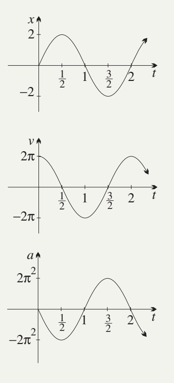
Step 2: Finding when at the origin (in interval $0 \leq t \leq 2$)

From the displacement graph, $x = 0$ when:

$t = 0, 1, 2$

At these times:

• When $t = 0$: speed = $2\pi$ m/s, acceleration = 0
• When $t = 1$: speed = $2\pi$ m/s, acceleration = 0
• When $t = 2$: speed = $2\pi$ m/s, acceleration = 0

Step 3: Finding when stationary (in interval $0 \leq t \leq 2$)

The particle is stationary when $v = 0$.

From the velocity graph: $t = \frac{1}{2}$ or $t = \frac{3}{2}$

At these times:

• When $t = \frac{1}{2}$: $x = 2$ metres, $a = -2\pi^2$ m/s²
• When $t = \frac{3}{2}$: $x = -2$ metres, $a = 2\pi^2$ m/s²

Step 4: Description of motion

The particle oscillates forever between $x = -2$ and $x = 2$, with period 2. It begins at the origin and moves first toward $x = 2$.

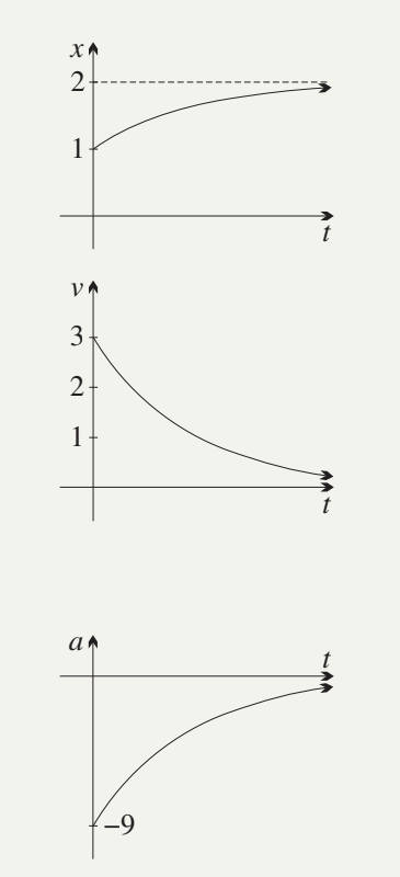
Worked Example: Exponential Motion with Limiting Values

A particle has height $x = 2 - e^{-3t}$ metres above ground at time $t$ seconds.

Step 1: Finding velocity and acceleration

$x = 2 - e^{-3t}$

$v = \frac{dx}{dt} = 3e^{-3t}$

$a = \frac{dv}{dt} = -9e^{-3t}$

Step 2: Initial values ($t = 0$)

Using $e^0 = 1$:

$x = 2 - 1 = 1 \text{ metre}$

$v = 3 \text{ m/s}$

$a = -9 \text{ m/s²}$

Step 3: Limiting values (as $t \to \infty$)

As $t$ increases, $e^{-3t} \to 0$

Therefore:

• $x \to 2$ metres
• $v \to 0$ m/s
• $a \to 0$ m/s²

Step 4: Description of motion

The particle starts 1 metre above the ground with initial velocity of 3 m/s upwards. It constantly slows down and moves toward a limiting position at height 2 metres, which it approaches but never quite reaches.