Further Applications of Differentiation Revision Notes for HSC SSCE Mathematics Advanced

Further Applications of Differentiation

Introduction

We can use differentiation to analyze and sketch graphs of functions that include $\log_e x$ . The derivative provides valuable information about tangents, normals, turning points, and the overall shape of logarithmic curves.

Finding tangents and normals to logarithmic curves

The derivative helps us find the equations of tangents and normals to curves involving logarithms. We use the key derivative:

chatImportant

The derivative of the natural logarithm is:

$\frac{d}{dx}(\log_e x) = \frac{1}{x}$

This derivative gives us the gradient of the tangent at any point on the curve $y = \log_e x$ .

lightbulbExample

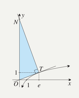
Worked Example: Tangent and normal to $y = \log_e x$ at $(e, 1)$

Let's find the tangent and normal to $y = \log_e x$ at the point $T(e, 1)$ .

Finding the tangent:

Differentiating gives us $\frac{dy}{dx} = \frac{1}{x}$

At point $T(e, 1)$ , the gradient is $\frac{1}{e}$

Using the point-gradient form:

$y - 1 = \frac{1}{e}(x - e)$

$ey - e = x - e$

$x = ey$

This can also be written as $y = \frac{x}{e}$

Notice that this tangent passes through the origin and has gradient $\frac{1}{e}$ .

Finding the normal:

Since the tangent has gradient $\frac{1}{e}$ , the normal has gradient $-e$ (negative reciprocal).

Using the point-gradient form:

$y - 1 = -e(x - e)$

$y = -ex + (e^2 + 1)$

Finding the area of the triangle:

Substituting $x = 0$ into the normal equation, we find the y-intercept is $N(0, e^2 + 1)$ .

The triangle $\triangle ONT$ has:

Base $ON = e^2 + 1$ (along the y-axis)
Altitude (height) $= e$ (horizontal distance from y-axis to point $T$ )

Area $= \frac{1}{2} \times e \times (e^2 + 1) = \frac{e(e^2 + 1)}{2}$ square units

Curve sketching with logarithmic functions

When sketching curves involving logarithmic functions, we follow a systematic approach to ensure we capture all important features of the graph.

infoNote

Six-Step Curve Sketching Process:

Write down the domain
Test whether the function is even, odd, or neither
Find any zeroes and examine the sign of the function
Examine the function's behaviour as $x \to \infty$ and as $x \to -\infty$
Find any stationary points and examine their nature
Find any points of inflection and examine the concavity

Following this systematic approach ensures you don't miss any important features when sketching logarithmic curves.

lightbulbExample

Worked Example: Sketching $y = x \log_e x$

Let's sketch the graph of $y = x \log_e x$ following this systematic approach.

Step 1: Domain

The function $\log_e x$ is only defined for $x > 0$ , so the domain is $x > 0$ .

Step 2: Even or odd?

The function is undefined when $x$ is negative, so it is neither even nor odd.

Step 3: Zeroes and sign

The only zero occurs when $x \log_e x = 0$ . Since $x > 0$ in the domain, we need $\log_e x = 0$ , which gives $x = 1$ .

To determine the sign of the function, we test values on either side of $x = 1$ :

When $x = e$ :

$y = e \log_e e = e \times 1 = e$ (positive)

When $x = e^{-1} = \frac{1}{e}$ :

$y = e^{-1} \log_e e^{-1} = \frac{1}{e} \times (-1) = -\frac{1}{e}$ (negative)

$x$	$0$	$e^{-1}$	$1$	$e$
$y$	*	$-e^{-1}$	$0$	$e$
sign	*	$-$	$0$	$+$

Therefore, $y$ is negative for $0 < x < 1$ and positive for $x > 1$ .

Step 4: Behaviour at limits

As given in the hint, $y \to 0$ as $x \to 0^+$ (we'll explain this limit behavior later).

Also, $y \to \infty$ as $x \to \infty$ because both $x$ and $\log_e x$ grow without bound.

Step 5: Stationary points

Using the product rule with $u = x$ and $v = \log_e x$ :

$u' = 1$ and $v' = \frac{1}{x}$

$f'(x) = vu' + uv' = \log_e x \times 1 + x \times \frac{1}{x}$

$f'(x) = \log_e x + 1$

For the second derivative:

$f''(x) = \frac{1}{x}$

Setting $f'(x) = 0$ :

$\log_e x + 1 = 0$

$\log_e x = -1$

$x = e^{-1}$

To determine the nature of this stationary point:

$f''(e^{-1}) = e > 0$ (positive, so it's a minimum)

$f(e^{-1}) = e^{-1} \times (-1) = -e^{-1}$

Therefore, $(e^{-1}, -e^{-1})$ is a minimum turning point.

An important observation: $f'(x) \to -\infty$ as $x \to 0^+$ , which means the curve becomes vertical (very steep) near the origin.

Step 6: Inflection points and concavity

Since $f''(x) = \frac{1}{x}$ is always positive for $x > 0$ , there are no inflection points.

The curve is always concave up throughout its domain.

The complete sketch:

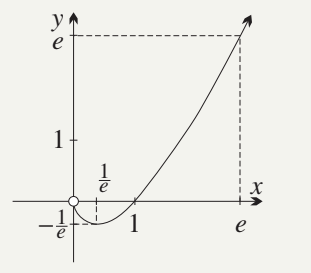
The graph shows a curve that:

Approaches the origin from below as $x \to 0^+$
Has a minimum turning point at $(e^{-1}, -e^{-1})$
Crosses the x-axis at $(1, 0)$
Increases without bound as $x \to \infty$
Is concave up throughout

Understanding limits involving logarithms

The limit of $x \log_e x$ as $x \to 0^+$

When examining the curve $y = x \log_e x$ near the origin, we face an interesting question. When $x$ is a small positive number, $\log_e x$ is a large negative number. So what happens to their product?

The answer is that $x \log_e x \to 0$ as $x \to 0^+$ . We say that $x$ dominates $\log_e x$ .

infoNote

This table demonstrates the behaviour as $x$ approaches zero from the right:

$x$	$\frac{1}{e}$	$\frac{1}{e^2}$	$\frac{1}{e^3}$	$\frac{1}{e^4}$	$\frac{1}{e^5}$	$\frac{1}{e^6}$	$\frac{1}{e^7}$
$x \log_e x$	$-\frac{1}{e}$	$-\frac{2}{e^2}$	$-\frac{3}{e^3}$	$-\frac{4}{e^4}$	$-\frac{5}{e^5}$	$-\frac{6}{e^6}$	$-\frac{7}{e^7}$
approx.	$-0.37$	$-0.27$	$-0.15$	$-0.073$	$-0.034$	$-0.015$	$-0.006$

As we can see, despite $\log_e x$ becoming more negative, the product approaches zero because $x$ is shrinking faster.

The limit of $\frac{\log_e x}{x}$ as $x \to \infty$

A similar issue arises when examining $\frac{\log_e x}{x}$ for large values of $x$ . Both the numerator and denominator grow without bound, so the behaviour is not immediately obvious.

Again, $x$ dominates $\log_e x$ , meaning that $\frac{\log_e x}{x} \to 0$ as $x \to \infty$ .

infoNote

This table illustrates the behaviour as $x$ grows without bound:

$x$	$e$	$e^2$	$e^3$	$e^4$	$e^5$	$e^6$	$e^7$
$\frac{\log_e x}{x}$	$\frac{1}{e}$	$\frac{2}{e^2}$	$\frac{3}{e^3}$	$\frac{4}{e^4}$	$\frac{5}{e^5}$	$\frac{6}{e^6}$	$\frac{7}{e^7}$
approx.	$0.37$	$0.27$	$0.15$	$0.073$	$0.034$	$0.015$	$0.006$

The table shows that although both numerator and denominator increase, the quotient approaches zero because the denominator grows faster.

The concept of domination

In both cases above, we say $x$ dominates $\log_e x$ . This is similar to how $e^x$ dominates $x$ (covered in earlier sections).

chatImportant

Understanding Domination:

This domination means:

In products where one term approaches zero and the other approaches infinity, the term approaching zero "wins"
In quotients where both terms approach infinity, the faster-growing term dominates

Key Limits: $\lim_{x \to 0^+} x \log_e x = 0$

$\lim_{x \to \infty} \frac{\log_e x}{x} = 0$

Exam tip: These limits are typically given in exam questions where needed. However, understanding the concept of domination helps you appreciate the behaviour of logarithmic functions.

bookmarkSummary

Key Points to Remember:

The derivative of $\log_e x$ is $\frac{1}{x}$ , which we use to find tangents and normals
When sketching logarithmic curves, follow the six-step process systematically: domain, symmetry, zeroes, behaviour at limits, stationary points, and concavity
Use the product rule when differentiating $x \log_e x$ : the result is $f'(x) = \log_e x + 1$
$x$ dominates $\log_e x$ : this means $x \log_e x \to 0$ as $x \to 0^+$ and $\frac{\log_e x}{x} \to 0$ as $x \to \infty$
Always check the second derivative to determine whether stationary points are maxima or minima, and to identify concavity

Further Applications of Differentiation (HSC SSCE Mathematics Advanced): Revision Notes