Applications of Differentiation (HSC SSCE Mathematics Advanced): Revision Notes
Applications of Differentiation
Introduction
Differentiation of trigonometric functions allows us to analyse many functions that are important in practical calculus applications. We can use these techniques to solve problems involving tangent lines, normal lines, and curve sketching. Additionally, differentiation helps us solve optimisation problems where we need to find maximum or minimum values.
Tangents and normals
When finding tangent and normal lines to trigonometric curves, we follow a systematic approach. First, we calculate the gradient at the relevant point by differentiating the function. Then we apply the point-gradient formula to find the equation of the line.
The point-gradient formula is essential for finding line equations:
where is the gradient and is the point on the curve.
For a normal line, remember that it is perpendicular to the tangent. Therefore, the gradient of the normal equals:
This perpendicular relationship is critical when solving geometry problems involving normals.
Finding the equation of a tangent line
Worked Example: Finding a Tangent to
Find the equation of the tangent to at the point where .
Step 1: Find the coordinates of the point.
When :
The point is .
Step 2: Find the gradient by differentiating.
Step 3: Evaluate the gradient at the point.
When :
Step 4: Apply the point-gradient formula.
Tangents and normals forming a square
Worked Example: Geometric Configuration with Tangents and Normals
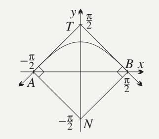
Consider the curve at the points and . Show that the tangents and normals at these points form a square.
Finding the gradients:
The derivative is:
At point :
Gradient of tangent
Gradient of normal
At point :
Gradient of tangent
Gradient of normal
Finding the equations:
Tangent at :
Normal at :
Tangent at :
Normal at :
Geometric properties:
The two tangents meet on the -axis at .
The two normals meet on the -axis at .
Since adjacent sides are perpendicular, is a rectangle. Since the diagonals are also perpendicular, it is a rhombus. Therefore, quadrilateral is a square.
Finding intercepts and calculating areas
Worked Example: Tangent Line and Triangle Area
Consider the tangent to at the point where . Find the intercepts and calculate the area of the triangle formed by the tangent and the coordinate axes.
Step 1: Find the point and gradient.
The function is .
Differentiating using the chain rule:
When :
Step 2: Find the tangent equation.
Step 3: Find the intercepts.
For the -intercept, set :
For the -intercept, set :
Step 4: Calculate the triangle area.
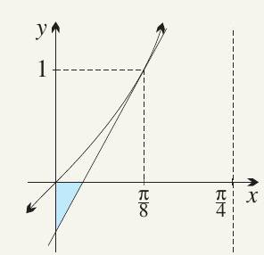
The tangent line and the coordinate axes form a triangle. Using the formula:
Note that , so:
Curve sketching
When sketching curves involving trigonometric functions, follow the systematic curve-sketching approach. The process can involve detailed calculations, but each step uses familiar techniques.
Exam Tip: Second Derivative Test
With trigonometric functions, checking the second derivative often provides a quicker and easier method to determine the nature of stationary points compared to using a table of first derivative values.
Using graphing technology (such as graphics calculators or computer software) can greatly improve understanding of how the equations relate to the shapes of these curves.
Sketching
Worked Example: Sketching
Sketch the curve for .
Step 1: Find values at domain endpoints.
When :
When :
Step 2: Find -intercepts.
Set :
(dividing by )
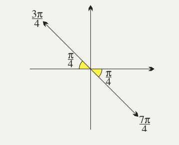
This means is in quadrant 2 or 4, with related angle .
Therefore: or
Step 3: Find stationary points.
Differentiate:
Set :
This means is in quadrant 1 or 3, with related angle .
Therefore: or
Step 4: Find the -values at stationary points.
When :
When :
Step 5: Determine the nature of stationary points using the second derivative.
When :
This is a maximum turning point at .
When :
This is a minimum turning point at .
Step 6: Find points of inflection.
The second derivative equals zero when:
These are the same values as the -intercepts: and .
We can verify the second derivative changes sign at these points by checking values:
The -intercepts and are also inflection points.
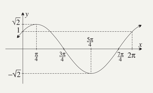
General Form: The final graph is a wave with the same period as and , but with amplitude . This function can be written as .
Any function of the form produces a similar wave pattern with modified amplitude and phase shift.
Sketching (harder example)
Practical Context: This function describes the area of a circular segment when the radius in the formula is held constant while the central angle varies.
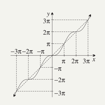
Worked Example: Sketching
Sketch the curve .
Step 1: Determine the domain.
The domain of is all real numbers.
Step 2: Test for symmetry.
Both and are odd functions.
Therefore, is odd, meaning .
The graph has rotational symmetry about the origin.
Step 3: Find zeroes and examine the sign.
The function equals zero at and nowhere else.
This is because:
- For : , so
- For : , so
Step 4: Examine behaviour as .
Since always remains between and :
As :
As :
Step 5: Find stationary points.
Differentiate:
Set :
This occurs at
Step 6: Determine the nature of stationary points.
Note that is never negative because always.
This means the curve is always increasing except at the stationary points.
At each stationary point:
- at these points
These are stationary inflection points:
Step 7: Find other points of inflection.
Differentiate again:
This equals zero at
Since changes sign around each of these points, the points are also inflection points.
At these inflection points:
The gradient at these additional inflection points is .
Key Points to Remember:
-
Finding tangents: Differentiate to get the gradient, then use point-gradient form to find the equation.
-
Finding normals: The normal is perpendicular to the tangent. If the tangent has gradient , the normal has gradient .
-
Second derivative test: For trigonometric functions, using the second derivative is often the quickest way to classify stationary points. If , it's a minimum; if , it's a maximum.
-
Curve sketching steps: Follow the systematic approach: domain, symmetry, intercepts, stationary points (first derivative), nature of stationary points (second derivative), inflection points (where second derivative changes sign), and end behaviour.
-
Functions like : These always produce wave patterns with the same period as and but with different amplitude and phase shift.