Graphing Linear Functions Revision Notes for HSC SSCE Mathematics Standard

Graphing Linear Functions

What is a linear function?

A linear function is a mathematical relationship between two variables that creates a straight line when graphed on a coordinate plane (also called a number plane). Linear functions are one of the most fundamental concepts in mathematics and appear frequently in real-world situations.

For example, the function $y = 3x$ is a linear function. It contains two variables: $y$ and $x$ . The beauty of linear functions is their predictability – they always produce a straight line when graphed.

infoNote

Linear functions appear everywhere in daily life! They can model relationships like:

Distance traveled over time at constant speed
Total cost based on price per item
Temperature conversion between Celsius and Fahrenheit
Earnings based on hourly wage

Understanding variables

When working with linear functions, it's important to understand the role of each variable:

Independent variable: This is the variable where you choose and substitute numbers. In most cases, this is $x$ . We call it "independent" because you can freely choose its value.

Dependent variable: This variable depends on the value you chose for the independent variable. In most cases, this is $y$ . Its value is determined by applying the function rule to the independent variable.

For example, in the function $y = 3x$ :

If we choose $x = 2$ (independent variable)
Then $y = 3 \times 2 = 6$ (dependent variable)
The value of $y$ depends on what we chose for $x$

infoNote

Think of it this way: the independent variable is the input you control, and the dependent variable is the output that results from that input. In most linear functions, $x$ represents the input and $y$ represents the output.

How to graph a linear function

Graphing a linear function is a systematic process that involves three main steps. Following these steps carefully will ensure you create an accurate graph every time.

Step 1: Create a table of values

Construct a table with two rows. The first row contains values for the independent variable (usually $x$ ), and the second row contains the corresponding values for the dependent variable (usually $y$ ). Choose several values for $x$ – typically at least five values work well, including negative numbers, zero, and positive numbers.

Step 2: Set up and plot points

Draw a coordinate plane with the independent variable on the horizontal axis and the dependent variable on the vertical axis. Then plot each coordinate pair from your table as a point on the plane. Be precise with your plotting to ensure accuracy.

Step 3: Join the points

Use a ruler to draw a straight line through all the plotted points. Extend the line beyond the points in both directions with arrows to show that the line continues infinitely. If your points don't line up perfectly, double-check your calculations.

chatImportant

Critical reminder: Always use a ruler when drawing your line! A freehand line may look straight to you, but small deviations can make your graph inaccurate. Also, if your plotted points don't line up perfectly, this indicates a calculation error – go back and check your table of values.

Worked example 1: Graphing a basic linear function

lightbulbExample

Worked Example: Graphing $y = 3x$

Let's graph the function $y = 3x$ .

Creating the table:

Choose five values for $x$ : $-2, -1, 0, 1,$ and $2$ . Calculate the corresponding $y$ values using the function $y = 3x$ :

$x$	$-2$	$-1$	$0$	$1$	$2$
$y$	$-6$	$-3$	$0$	$3$	$6$

Setting up the coordinate plane:

Draw a coordinate plane with $x$ on the horizontal axis and $y$ on the vertical axis.

Plotting the points:

Plot these coordinate pairs: $(-2, -6)$ , $(-1, -3)$ , $(0, 0)$ , $(1, 3)$ , and $(2, 6)$ .

Drawing the line:

Join all the points with a straight line extending in both directions.

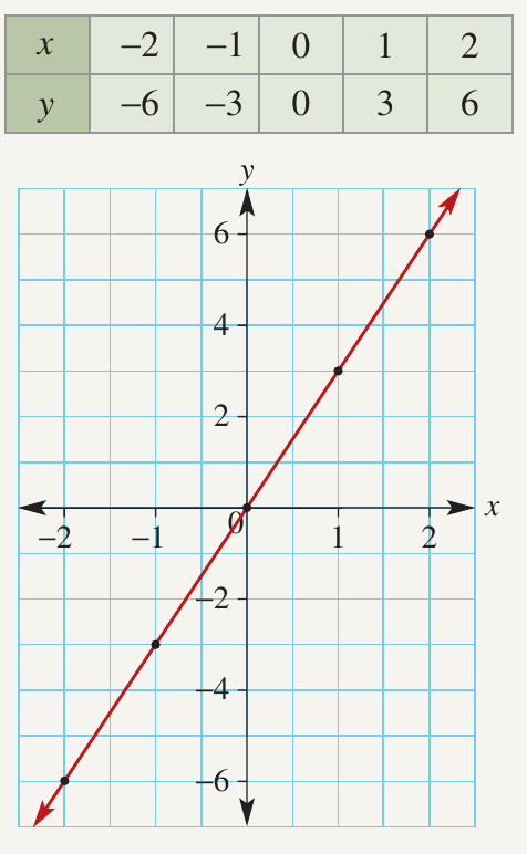
Notice how this line passes through the origin $(0, 0)$ and has a positive slope, meaning it rises as you move from left to right.

Worked example 2: Graphing a linear function with a y-intercept

lightbulbExample

Worked Example: Graphing $y = 2x - 1$

Now let's graph the function $y = 2x - 1$ .

Creating the table:

Choose five values for $x$ : $-2, -1, 0, 1,$ and $2$ . Calculate the corresponding $y$ values using the function $y = 2x - 1$ :

$x$	$-2$	$-1$	$0$	$1$	$2$
$y$	$-5$	$-3$	$-1$	$1$	$3$

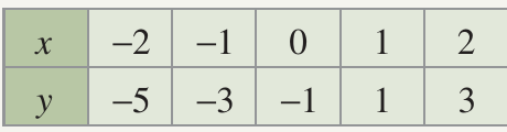
Setting up the coordinate plane:

Draw a coordinate plane with $x$ on the horizontal axis and $y$ on the vertical axis.

Plotting the points:

Plot these coordinate pairs: $(-2, -5)$ , $(-1, -3)$ , $(0, -1)$ , $(1, 1)$ , and $(2, 3)$ .

Drawing the line:

Join all the points with a straight line extending in both directions.

This line has a positive slope but crosses the $y$ -axis at $-1$ rather than at the origin. The $-1$ in the equation represents where the line intersects the $y$ -axis.

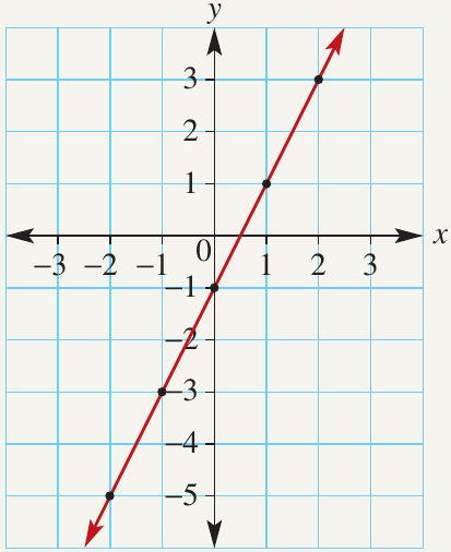
Worked example 3: Graphing a linear function with negative slope

lightbulbExample

Worked Example: Graphing $y = -x - 2$

Finally, let's graph the function $y = -x - 2$ .

Creating the table:

Choose five values for $x$ : $-2, -1, 0, 1,$ and $2$ . Calculate the corresponding $y$ values using the function $y = -x - 2$ :

$x$	$-2$	$-1$	$0$	$1$	$2$
$y$	$0$	$-1$	$-2$	$-3$	$-4$

Setting up the coordinate plane:

Draw a coordinate plane with $x$ on the horizontal axis and $y$ on the vertical axis.

Plotting the points:

Plot these coordinate pairs: $(-2, 0)$ , $(-1, -1)$ , $(0, -2)$ , $(1, -3)$ , and $(2, -4)$ .

Drawing the line:

Join all the points with a straight line extending in both directions.

Notice how this line has a negative slope, meaning it falls as you move from left to right. The negative sign in front of $x$ creates this downward slope.

Exam tips

infoNote

Tips for Success:

Always use a ruler to draw your lines – freehand lines may not be accurate enough
Choose a good range of $x$ values including negative numbers, zero, and positive numbers
Check that all your points line up before drawing the final line
Extend your line with arrows at both ends to show it continues infinitely
Label your axes clearly with $x$ and $y$
If possible, include the origin in your coordinate plane as it's a helpful reference point

Remember!

bookmarkSummary

Key Points to Remember:

A linear function always creates a straight line when graphed on a coordinate plane
The independent variable (usually $x$ ) goes on the horizontal axis, and the dependent variable (usually $y$ ) goes on the vertical axis
Create a table of values by choosing several $x$ values and calculating the corresponding $y$ values using the function rule
Plot all points carefully and use a ruler to join them with a straight line
Positive coefficients of $x$ create upward-sloping lines (from left to right), while negative coefficients create downward-sloping lines

Graphing Linear Functions (HSC SSCE Mathematics Standard): Revision Notes