Using Excel to Model an Annuity Revision Notes for HSC SSCE Mathematics Standard

Using Excel to Model an Annuity

Excel provides powerful built-in functions specifically designed to work with annuities. These functions automate complex calculations involving regular payments and compound interest, making it much easier to solve financial problems. Instead of manually calculating compound interest for each payment period, you can use Excel's financial functions to get accurate results quickly.

Excel financial functions for annuities

Excel offers five main functions for annuity calculations. Each function calculates a different aspect of an annuity, depending on what information you have and what you need to find.

The five key functions are:

FV (Future Value): Calculates the total value of an investment after making regular payments with compound interest
PV (Present Value): Calculates what a series of future payments is worth today
NPER (Number of Periods): Calculates how many payment periods are needed to reach a goal
PMT (Payment): Calculates the regular payment amount needed
RATE (Interest Rate): Calculates the interest rate per period

Function syntax

Each Excel function follows a specific format with required and optional arguments:

Future Value: = FV(rate, nper, pmt, [pv], [type])

Present Value: = PV(rate, nper, pmt, [fv], [type])

Number of Periods: = NPER(rate, pmt, pv, [fv], [type])

Payment: = PMT(rate, nper, pv, [fv], [type])

Interest Rate: = RATE(nper, pmt, pv, [fv], [type], [guess])

infoNote

Arguments shown in square brackets [pv], [fv], [type] are optional. You only need to include them when they're relevant to your calculation.

Understanding function arguments

To use Excel's financial functions correctly, you need to understand what each argument represents. These arguments are the inputs you provide to the function.

Rate

The interest rate per period, expressed as a decimal. For example, $10\%$ is entered as $0.10$ .

chatImportant

The rate must match your payment period. If you're making monthly payments, convert the annual interest rate to a monthly rate by dividing by $12$ . For example, $6\%$ per annum becomes $\frac{0.06}{12} = 0.005$ per month.

Nper

The total number of payment periods in the annuity. This is how many times you will make a payment.

If payments are made monthly for $3$ years, then $\text{nper} = 3 \times 12 = 36$ months.

Pmt

The payment made each period. This amount must remain constant throughout the life of the annuity.

chatImportant

Excel convention: Enter payments as negative values. This is because payments represent money leaving your account. For example, a $250 monthly payment is entered as $-250$ .

Pv

Present value, which is the current lump sum amount. This represents how much a series of future payments is worth right now, or it could be an initial investment amount.

Fv

Future value, which is the total amount you will have after all payments and interest are accumulated. This is the sum of all contributions plus compound interest earned.

Type

Indicates when payments are made:

Type $= 0$ : Payments are due at the end of each period (most common)
Type $= 1$ : Payments are due at the beginning of each period

infoNote

If you don't specify type, Excel assumes payments are made at the end of the period.

Guess

An estimated value for the interest rate, used only with the RATE function. Excel uses this as a starting point for its calculations. If you don't provide a guess, Excel uses $0.1$ ( $10\%$ ) as the default.

Calculating future value

The FV function calculates how much money you will have in the future after making regular payments with compound interest. This is useful when planning savings goals.

lightbulbExample

Worked Example: Ella's Cruise Savings

Question: Ella wants to save for a cruise. She will invest $250 at the end of each month into an account earning $6.4\%$ per annum compounded monthly. She will do this for three years. How much will Ella have for her cruise?

Solution:

Step 1: Identify the Excel function needed

To find the future value, use the FV function.

Step 2: Determine the compounding period

The investment compounds monthly, so all arguments must be expressed per month.

Step 3: Calculate the interest rate per period

The annual rate is $6.4\% = 0.064$

For monthly compounding:

$\text{RATE} = \frac{0.064}{12}$

Step 4: Calculate the number of periods

Number of months in $3$ years:

$\text{NPER} = 3 \times 12 = 36$

Step 5: Enter the payment as a negative value

Monthly payment:

$\text{PMT} = -250$

(Negative because money is leaving Ella's account)

Step 6: Enter the formula in Excel

In cell A1, type:

= FV((0.064/12), 36, -250)

Step 7: Calculate the result

Press Enter to view the answer: $9893.09

Answer: The future value is $9893.09. Ella will have $9893.09 for her cruise.

infoNote

Exam tip: Always check that your interest rate matches your payment period. Annual rates must be divided by the number of payments per year.

Calculating payment amount

The PMT function calculates the regular payment you need to make to reach a specific future value or to pay off a present value. This is useful when you have a savings target and want to know how much to contribute each period.

lightbulbExample

Worked Example: Angus's Investment

Question: Angus plans to invest into an annuity at the end of each year that pays $10\%$ per annum compound interest. Calculate the annual payment Angus needs to make to have $10,000 at the end of $4$ years.

Solution:

Step 1: Identify the Excel function needed

To find the payment amount, use the PMT function.

Step 2: Determine the compounding period

The investment compounds annually (per year), so arguments are per annum.

Step 3: Express the interest rate as a decimal

$\text{RATE} = 10\% = 0.10$

Step 4: Determine the number of periods

$\text{NPER} = 4 \text{ years}$

Step 5: Enter the future value as a negative

Target amount (future value):

$\text{FV} = -10000$

(Negative because we're working backwards from the goal)

Step 6: Enter the formula in Excel

In cell A1, type:

= PMT(0.10, 4, 0, -10000)

Note: The present value (pv) is $0$ because there's no initial lump sum.

Step 7: Calculate the result

Press Enter to view the answer: $2154.71

Answer: The payment is $2154.71. Angus needs to invest $2154.71 each year.

Spreadsheet demonstration

The example below shows how the PMT calculation appears in a spreadsheet with labeled cells:

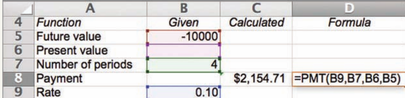
Notice how the spreadsheet organizes the information:

Column A: Function labels (Future value, Present value, etc.)
Column B: Given values (inputs)
Column C: Calculated results
Column D: The Excel formula used

infoNote

The formula =PMT(B9,B7,B6,B5) references the cells containing rate, nper, pv, and fv values.

Calculating present value

The PV function calculates the present value of an annuity. This tells you what a series of future payments is worth in today's money. Present value is important for comparing investment options or understanding the current worth of future cash flows.

lightbulbExample

Worked Example: Present Value Calculation

Question: Find the present value of an annuity in which $1300 is invested at a rate of $5.8\%$ p.a. compounded annually at the end of every year for $6$ years.

Solution:

Step 1: Identify the Excel function needed

To find the present value, use the PV function.

Step 2: Determine the compounding period

The investment compounds annually (every year), so arguments are per annum.

Step 3: Express the interest rate as a decimal

$\text{RATE} = 5.8\% = 0.058$

Step 4: Determine the number of periods

$\text{NPER} = 6 \text{ years}$

Step 5: Enter the payment as a negative value

Annual payment:

$\text{PMT} = -1300$

Step 6: Enter the formula in Excel

In cell A1, type:

= PV(0.058, 6, -1300)

Step 7: Calculate the result

Press Enter to view the answer.

Answer: The present value is $6432.89. The series of six annual $1300 payments is worth $6432.89 in today's money.

Spreadsheet demonstration

The example below shows the PV calculation in spreadsheet format:

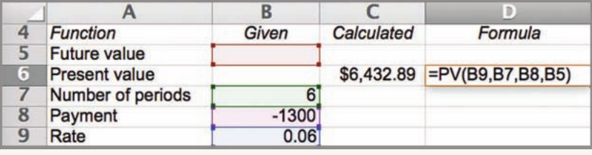
The spreadsheet shows:

Row 6: Present value result of $6432.89
Row 7: Number of periods = $6$
Row 8: Payment = $-1300$
Row 9: Rate = $0.06$ (which should be $0.058$ as per the problem, but the image shows $0.06$ )
Column D: The formula =PV(B9,B7,B8,B5) showing cell references

Key Excel conventions for financial functions

When working with Excel's financial functions, follow these important conventions:

chatImportant

Critical Conventions to Remember:

1. Express interest rates as decimals

Convert percentages by dividing by $100$ . For example: $10\% = 0.10$

2. Match rate to payment period

If making monthly payments with an annual interest rate, divide the annual rate by $12$ .

3. Use negative values for money going out

Regular payments and lump sum deposits are entered as negative numbers.

4. Use negative values for target amounts

When calculating payments needed to reach a goal, enter the goal (future value) as negative.

5. Specify all required arguments

Each function needs specific inputs in the correct order. Optional arguments can be omitted if not relevant.

bookmarkSummary

Key Points to Remember:

Excel has five main financial functions: FV (future value), PV (present value), PMT (payment), NPER (number of periods), and RATE (interest rate)
Always convert percentages to decimals: For example, $6.4\%$ becomes $0.064$ in Excel formulas
Match your rate to your payment period: Annual interest rates must be divided by the number of payments per year (e.g., divide by $12$ for monthly payments, divide by $4$ for quarterly payments)
Enter payments as negative values: Money leaving your account is negative in Excel. This includes regular payments and sometimes target amounts when working backwards
The order of arguments matters: Each function requires arguments in a specific sequence. Make sure you enter rate, nper, pmt, pv, and fv in the correct positions

Using Excel to Model an Annuity (HSC SSCE Mathematics Standard): Revision Notes