Interpolation and Extrapolation (HSC SSCE Mathematics Standard): Revision Notes
Interpolation and Extrapolation
Understanding the regression line
The regression line (also called the line of best fit) is a powerful tool that reveals key information about the relationship between variables and enables us to make predictions.
The regression line equation provides two important pieces of information:
- Gradient (m): This tells us how much the dependent variable changes each time the independent variable increases by one unit. It represents the rate of change in the relationship.
- Vertical intercept (b): This shows the value of the dependent variable when the independent variable equals zero. It represents the starting point of the relationship.
Think of the gradient as the "steepness" of your line - it tells you how quickly one variable changes in response to the other. The vertical intercept is where your line crosses the y-axis, showing the starting value before any changes occur.
Beyond providing this information, the regression line equation is essential for two key prediction techniques: interpolation and extrapolation.
What is interpolation?
Interpolation means using the regression line to estimate values that fall within the boundaries of your existing data.
When you interpolate, you're making predictions for values that lie between the data points you've already collected. Think of it as filling in the blanks within your dataset.
Confidence in interpolation
The reliability of your interpolated predictions depends on the strength of the linear association:
- Strong linear association: When data points show a strong linear pattern, we can trust our predictions to be quite accurate.
- Weak linear association: When the linear pattern is weak, our confidence in the predictions decreases.
Key principle: If the data has a strong linear association, then we can be confident our predictions are accurate. However, if the data has a weak linear association, we are less confident with our predictions.
Worked example: Life expectancy predictions
Let's look at how interpolation works using life expectancy data for females and males from 1910 to 2010.
Data:
| Year | 1910 | 1920 | 1930 | 1940 | 1950 | 1960 | 1970 | 1980 | 1990 | 2000 | 2010 |
|---|---|---|---|---|---|---|---|---|---|---|---|
| Female | 58 | 63 | 66 | 68 | 70 | 72 | 74 | 76 | 79 | 82 | 84 |
| Male | 55 | 59 | 62 | 63 | 65 | 67 | 66 | 68 | 73 | 77 | 79 |
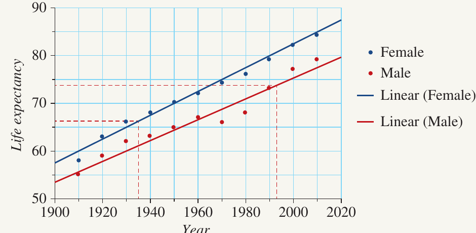
Worked Example: Predicting Life Expectancy Using Interpolation
Question a: What was the life expectancy in 1935 for females?
Solution:
To find the life expectancy for females in 1935:
- Draw a vertical line from 1935 on the horizontal axis until it intersects the blue line (female trend line)
- From this intersection point, draw a horizontal line to the vertical axis
- Read the value where the horizontal line meets the vertical axis
Answer: Life expectancy for females in 1935 is approximately 67 years.
Question b: What was the life expectancy in 1995 for males?
Solution:
To find the life expectancy for males in 1995:
- Draw a vertical line from 1995 on the horizontal axis until it intersects the red line (male trend line)
- From this intersection point, draw a horizontal line to the vertical axis
- Read the value where the horizontal line meets the vertical axis
Answer: Life expectancy for males in 1995 is approximately 74 years.
Note: Both 1935 and 1995 fall within the range of our dataset (1910-2010), so these are interpolation examples. The predictions are reliable because the data shows a strong linear association.
What is extrapolation?
Extrapolation involves extending the regression line to predict values beyond the range of your collected data.
When you extrapolate, you're making predictions for values that are either smaller or larger than any values in your dataset. Think of it as drawing the line further past your last data point.
Important caution about extrapolation
While extrapolation can be useful, it requires careful consideration. The accuracy of extrapolated predictions depends on the strength of the linear association, similar to interpolation. However, there's an additional concern: extending predictions too far beyond your data can lead to unrealistic results.
The further you extrapolate from your data, the less reliable your predictions become. This happens because the relationship that exists within your dataset may not continue unchanged outside that range. Real-world factors often cause relationships to change beyond the boundaries of your observations.
Worked example: Height predictions
Let's examine how extrapolation works using height and age data for a student.
Data:
| Age (in years) | 7 | 8 | 9 | 10 | 11 | 12 | 13 | 14 | 15 | 16 |
|---|---|---|---|---|---|---|---|---|---|---|
| Height (in cm) | 133 | 139 | 144 | 149 | 156 | 163 | 170 | 174 | 177 | 181 |
Worked Example: Understanding the Limitations of Extrapolation
Question a: Construct a scatterplot from the table using age from 0 to 30 and height from 100 to 300.
Solution:
- Create a scatterplot with age on the horizontal axis (0 to 30 years)
- Place height on the vertical axis (100 to 300 cm)
- Plot each data point from the table
- For example, plot (7, 133), (8, 139), (9, 144), and so on
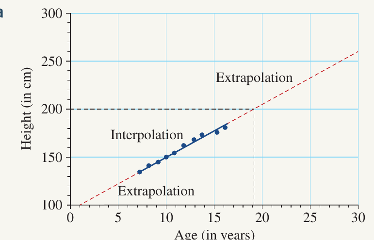
Question b: Draw the line of best fit and describe the association between age and height.
Solution:
The scatterplot shows only a small amount of scatter in the data points.
Answer: Strong positive linear association.
Question c: Predict the height of the student when they are aged 19 years.
Solution:
To predict the height at age 19:
- Locate 19 on the horizontal axis
- Draw a vertical line up to the regression line
- From the intersection, draw a horizontal line to the vertical axis
- Read the height value
Answer: Height of the student is 200 cm when they are 19 years old.
Note: Age 19 is outside our dataset range (7-16 years), so this is extrapolation.
Question d: What are the limitations of this linear model?
Solution:
This question highlights a crucial limitation of extrapolation.
Answer: Adult height does not grow at the same rate as a child. Using the model to extrapolate is flawed. For example, the prediction suggests the height will be 260 cm at age 30, which is unrealistic.
Key insight: While children grow rapidly and steadily during their developing years, growth slows and eventually stops in adulthood. The linear relationship that exists for ages 7-16 does not continue beyond this range. This demonstrates why we must be cautious when extrapolating, especially when extending far beyond our dataset.
Common Mistake to Avoid: Don't assume that linear patterns continue indefinitely. Real-world relationships often change outside the observed range. Always ask yourself: "Is it reasonable to assume this pattern continues beyond my data?"
Comparing interpolation and extrapolation
Understanding the key difference between these two techniques is essential for making reliable predictions:
| Interpolation | Extrapolation |
|---|---|
| Predicting values within the dataset range | Predicting values outside the dataset range |
| Generally more reliable | Requires more caution |
| "Filling in the gaps" between known points | "Extending the pattern" beyond known points |
Exam tip: Remember that interpolation is typically more reliable than extrapolation because you're working within known territory. When extrapolating, always consider whether the relationship is likely to continue unchanged beyond your data range.
Remember!
Key Points to Remember:
-
Interpolation means predicting values within your dataset range - it's like filling in the gaps between your data points.
-
Extrapolation means predicting values outside your dataset range - it's like extending the line beyond your last data point, which requires caution.
-
Strong linear associations lead to more confident and accurate predictions for both interpolation and extrapolation.
-
The further you go, the less you know - the further you extrapolate from your data, the less reliable your predictions become because relationships may change beyond the observed range.
-
Always consider real-world factors when extrapolating - linear patterns don't always continue indefinitely (like the height example, where growth stops in adulthood).
Memory aids:
- INTER-polation = INTERNAL (within the data range)
- EXTRA-polation = EXTRA territory (outside the data range)