Line of Best Fit (HSC SSCE Mathematics Standard): Revision Notes
Line of Best Fit
Introduction
When we examine bivariate data on a scatterplot, we often see patterns that suggest a relationship between the two variables. If the points tend to follow a straight line pattern, we can draw a line through the data to represent this relationship. This line is called the line of best fit.
A line of best fit is a straight line that best approximates the linear relationship between data points on a scatterplot. The process of finding this line is called linear regression.
The equation of a line of best fit follows the familiar gradient-intercept form:
where:
- is the gradient (or slope) of the line
- is the y-intercept
Lines of best fit are powerful tools used in many fields, from predicting sales trends in business to modeling climate change in environmental science. They help us understand relationships between variables and make informed predictions.
Using the line of best fit for predictions
Once we have established a line of best fit, we can use it to make predictions about one variable based on the other. There are two types of predictions:
Interpolation occurs when we make a prediction within the existing data range. This is generally more reliable because we are working within the boundaries of our observed data.
Extrapolation occurs when we make a prediction outside the existing data range. We must use this cautiously because the linear relationship we observed may not continue beyond our data.
Be Very Careful with Extrapolation!
Always question whether the relationship would continue outside your data range. For example, predicting an adult's height based on their childhood growth pattern would be unreliable extrapolation, as growth patterns change dramatically after puberty. The relationship that holds within your data may break down outside it.
Method of least squares
Why we need a systematic method
If we simply tried to draw a line that appears to balance the points above and below it, different people would likely draw slightly different lines. This subjective approach is not reliable for scientific analysis. We need a systematic mathematical method that produces the same result every time.
Understanding residuals
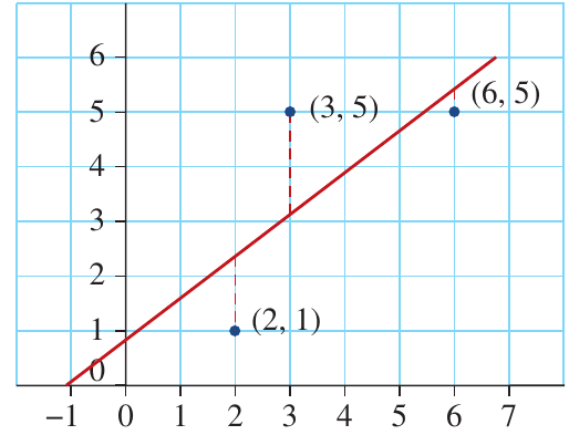
For any line drawn through a scatterplot, we can measure how well it fits the data by calculating the vertical distance from each point to the line. This vertical distance is called a residual.
A residual measures how far a data point is from the line:
- If the line passes exactly through a point, the residual is zero
- The larger the residual, the worse the fit for that particular point
The least-squares approach
The least-squares line of best fit is the line that minimizes the sum of all squared residuals. Here's how it works:
- Calculate the residual (vertical distance) for each data point
- Square each residual value
- Add all the squared values together
- The best line is the one that makes this total as small as possible
By squaring the residuals, we ensure that:
- Negative and positive distances don't cancel out
- Larger errors are penalized more heavily than smaller ones
Why This Method is Reliable
This mathematical approach guarantees that everyone analyzing the same data will arrive at the same line of best fit. There's no guesswork or subjective judgment—the mathematics determines the optimal line objectively and consistently.
Calculating the equation of the least-squares line
To find the equation of the least-squares line of best fit, we need five statistical measures from our data:
- = mean of the values
- = mean of the values
- = standard deviation of the values
- = standard deviation of the values
- = Pearson's correlation coefficient
Formula for the gradient
The gradient (slope) of the line is calculated using:
This formula shows that:
- The gradient depends on the correlation strength ()
- It's adjusted by the ratio of standard deviations
- A stronger correlation produces a steeper gradient
Formula for the y-intercept
Once we have the gradient, we calculate the y-intercept using:
This ensures the line passes through the point , which is the centre of the data.
Understanding the Variables
- represents the gradient (how steep the line is)
- represents where the line crosses the y-axis
- must be between and (this is the correlation coefficient)
- and measure the spread of the data
- and are the average values
The line of best fit will always pass through the point —you can use this to check your work!
Complete equation
Combining these, the equation of the least-squares line of best fit is:
where and
Worked example 1: Calculating from given statistics
Worked Example: Finding the Line of Best Fit from Statistics
Question: The heights () and masses () of nine people have been recorded. The following statistics were calculated: , , , , and .
Calculate the gradient, y-intercept, and equation of the least-squares line of best fit.
Solution:
Part a) Calculate the gradient:
Write the gradient formula:
Substitute the values:
Calculate:
Part b) Calculate the y-intercept:
Write the y-intercept formula:
Substitute the values:
Calculate:
Part c) Write the equation:
Start with the gradient-intercept form:
Substitute our calculated values:
Express using variable names:
Interpretation: This equation tells us that for every cm increase in height, mass increases by approximately kg.
Worked example 2: Complete analysis with data
Worked Example: Complete Analysis from Data Table
Question: The table below shows the heights (cm) and masses (kg) of nine people.
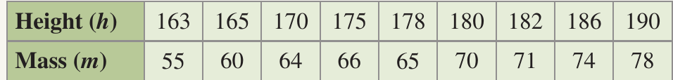
Find Pearson's correlation coefficient, determine the equation of the least-squares line of best fit using a calculator, draw the scatterplot with the line, and describe the association.
Solution:
Part a) Find Pearson's correlation coefficient:
Using a calculator in statistics mode with the data entered:
This indicates a very strong positive correlation between height and mass.
Part b) Determine the equation:
Using calculator regression functions:
Write the gradient-intercept formula:
Substitute the calculator values:
Part c) Draw the scatterplot:
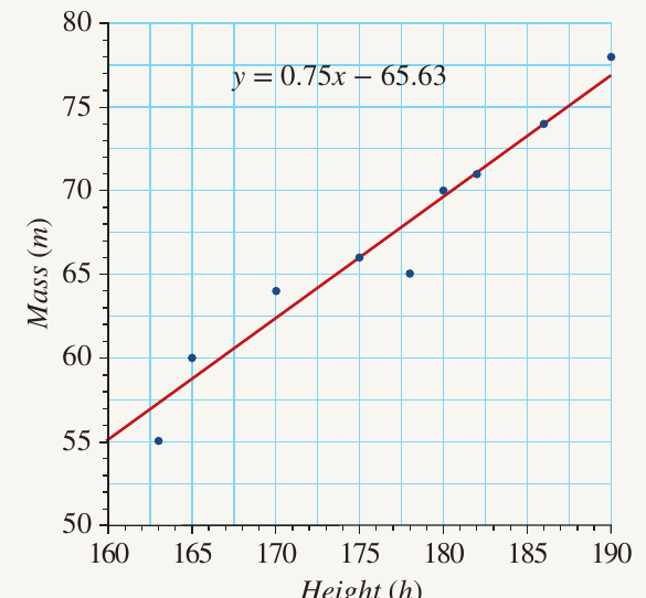
To draw the line accurately:
Step 1: Select two values within the data range (e.g., and )
Step 2: For :
Plot the point
Step 3: For :
Plot the point
Step 4: Draw a straight line through these two points, extending across the data range.
Part d) Describe the association:
Since Pearson's correlation coefficient is between and , we describe this as:
Strong positive linear association
Interpretation: This means that as height increases, mass tends to increase in a very predictable linear pattern.
Exam tips
Tips for Success in Exams
- Always show your working when calculating gradient and y-intercept
- Round final answers appropriately (usually to decimal places)
- When describing association, mention three things: strength (weak/moderate/strong), direction (positive/negative), and type (linear)
- Check your line of best fit passes through or near the mean point
- Be cautious about extrapolation—always consider whether the relationship would continue outside the data range
Remember!
Key Points to Remember:
-
A line of best fit is a straight line that best represents the linear relationship between two variables, with equation
-
The least-squares method finds the line that minimizes the sum of squared residuals (vertical distances from points to the line)
-
Calculate the gradient using:
-
Calculate the y-intercept using:
-
Interpolation (predicting within the data range) is reliable, but extrapolation (predicting outside the range) must be used cautiously
-
The correlation coefficient indicates the strength and direction of the relationship—use it to describe the association
-
The line of best fit always passes through the centre point of the data