Linear Functions Revision Notes for HSC SSCE Mathematics Standard

Linear Functions

What are linear functions?

A linear function creates a straight line when you graph it on a coordinate plane. These functions involve two variables, typically $x$ and $y$ , that have a special relationship.

infoNote

Understanding variables:

When working with linear functions like $y = 3x - 2$ , we have two types of variables:

Independent variable: This is the variable you choose a value for (usually $x$ ). You have control over this value.
Dependent variable: This is the variable whose value depends on what you chose for the independent variable (usually $y$ ). It changes based on the independent variable.

For example, in the function $y = 3x - 2$ , if we choose $x = 2$ (independent), then $y = 3 \times 2 - 2 = 4$ (dependent). The value of $y$ depends on the value we selected for $x$ .

Graphing linear functions

To draw the graph of a linear function, follow these steps:

Step 1: Create a table of values

Set up a table with the independent variable ( $x$ ) in the first row and the dependent variable ( $y$ ) in the second row. Choose several values for $x$ (usually including negative numbers, zero, and positive numbers).

Step 2: Set up your coordinate plane

Draw a number plane with:

The independent variable ( $x$ ) on the horizontal axis
The dependent variable ( $y$ ) on the vertical axis

Then plot all the points from your table.

Step 3: Draw the line

Join all the plotted points with a straight line. Extend the line beyond your points with arrows to show it continues infinitely in both directions.

lightbulbExample

Worked Example: Drawing a linear function

Let's draw the graph of $y = -2x - 1$ .

Solution:

First, create a table of values for $x$ and $y$ :

$x$	$-2$	$-1$	$0$	$1$	$2$
$y$	$3$	$1$	$-1$	$-3$	$-5$

To find each $y$ value, substitute the $x$ value into the equation $y = -2x - 1$ .

For example, when $x = -2$ :

y = -2(-2) - 1

y = 4 - 1

y = 3

Plot the points $(-2, 3)$ , $(-1, 1)$ , $(0, -1)$ , and $(1, -3)$ on your coordinate plane.

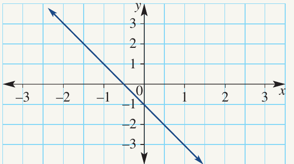
Join these points with a straight line extending in both directions.

chatImportant

Exam tip: Choose $x$ values that are evenly spaced and include both positive and negative numbers as well as zero. This helps create an accurate graph.

The gradient-intercept formula

The gradient-intercept formula is a special way of writing the equation of a straight line. It takes the form:

$y = mx + c$

In this formula:

$m$ represents the gradient (also called the slope)
$c$ represents the y-intercept

infoNote

Understanding gradient:

The gradient tells us how steep the line is. It measures the slope of the line by comparing vertical change to horizontal change.

$\text{Gradient (m)} = \frac{\text{Vertical rise}}{\text{Horizontal run}}$

Types of gradients:

Positive gradient: Lines that slope upward to the right (/) have positive gradients
Negative gradient: Lines that slope downward to the right () have negative gradients

The larger the absolute value of the gradient, the steeper the line.

infoNote

Understanding y-intercept:

The y-intercept is where the line crosses the vertical ( $y$ ) axis. It's the value of $y$ when $x = 0$ . In the formula $y = mx + c$ , the value of $c$ gives you this intercept directly.

lightbulbExample

Worked Example: Finding gradient and y-intercept from a graph

Draw the graph of $y = 3x - 2$ from a table of values. Find the gradient and y-intercept of this line.

Solution:

Create a table of values:

$x$	$-2$	$-1$	$0$	$1$	$2$
$y$	$-8$	$-5$	$-2$	$1$	$4$

Plot the points $(-1, -5)$ , $(0, -2)$ , $(1, 1)$ , and $(2, 4)$ .

Join the points to make a straight line.

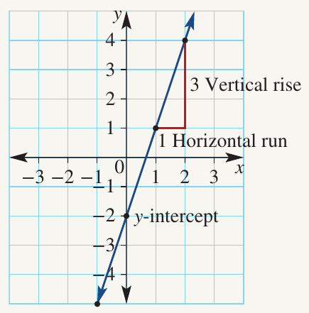
To find the gradient, use the rise over run formula:

Choose two clear points on your line.

Count the vertical rise: $3$ units

Count the horizontal run: $1$ unit

Therefore:

$m = \frac{3}{1} = 3$

To find the y-intercept, identify where the line crosses the y-axis:

The line crosses at $(0, -2)$

Therefore: $c = -2$

Write the equation:

$y = 3x - 2$

This matches our original equation, confirming our gradient and y-intercept are correct.

Sketching using gradient and y-intercept

When an equation is already written in the form $y = mx + c$ , you can sketch the line quickly without creating a full table of values. You only need two points: the y-intercept and one other point found using the gradient.

infoNote

Quick sketching method:

Rearrange the equation (if needed) into the form $y = mx + c$
Identify the gradient ( $m$ ) and y-intercept ( $c$ )
Plot the y-intercept on the y-axis
Use the gradient to find a second point
Draw a straight line through both points

lightbulbExample

Worked Example: Sketching from gradient and y-intercept

Sketch the graph of $3y + 6x = 9$ .

Solution:

First, rearrange into gradient-intercept form:

$3y + 6x = 9$

Subtract $6x$ from both sides:

$3y = 9 - 6x$

Divide both sides by $3$ :

$y = \frac{9 - 6x}{3}$

Simplify:

$y = 3 - 2x$

Rewrite in standard form:

$y = -2x + 3$

Identify gradient and y-intercept:

Gradient: $m = -2$

Y-intercept: $c = 3$

Plot the y-intercept at point $(0, 3)$ .

Use the gradient to find the second point:

A gradient of $-2$ means $\frac{-2}{1}$ (down $2$ , across $1$ )

From $(0, 3)$ , move $1$ unit right and $2$ units down.

This gives the point $(1, 1)$ .

Draw a straight line through $(0, 3)$ and $(1, 1)$ .

chatImportant

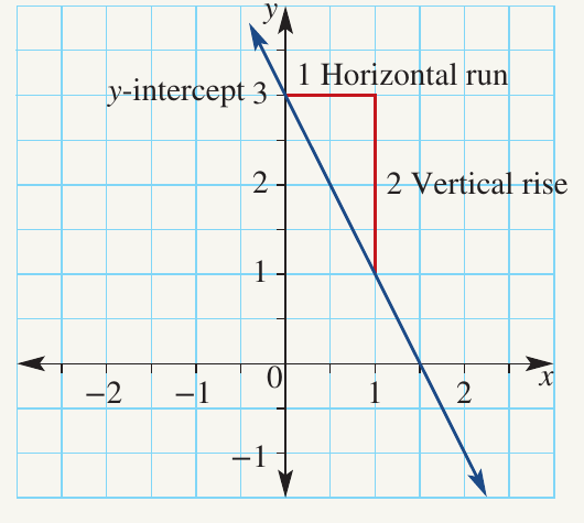
Exam tip: With negative gradients, remember to move down (in the negative y-direction) as you move right (in the positive x-direction).

Parallel lines

Two or more lines are parallel if they never intersect (cross each other), no matter how far they are extended. In coordinate geometry, we can identify parallel lines by examining their gradients.

infoNote

Condition for parallel lines:

Lines are parallel when they have the same gradient. If two linear functions have the same value of $m$ , their graphs will be parallel lines.

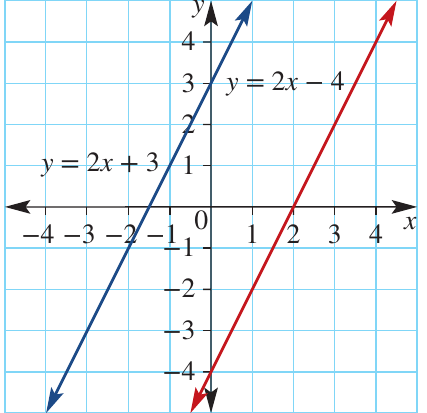
Example: Identifying parallel lines

Consider these two linear functions:

$y = 2x + 3$ has gradient $m = 2$ and y-intercept $c = 3$
$y = 2x - 4$ has gradient $m = 2$ and y-intercept $c = -4$

Both lines have a gradient of $2$ , so they are parallel. They have different y-intercepts ( $3$ and $-4$ ), which means they cross the y-axis at different points, but they maintain the same steepness throughout and will never meet.

infoNote

Key point: Parallel lines run in the same direction with identical steepness but start at different positions on the y-axis.

bookmarkSummary

Key Points to Remember:

A linear function creates a straight line on a coordinate plane and has the form $y = mx + c$
The gradient ( $m$ ) shows the steepness of the line and is calculated as $\frac{\text{rise}}{\text{run}}$
The y-intercept ( $c$ ) shows where the line crosses the y-axis
Positive gradients slope upward to the right (/), while negative gradients slope downward to the right ()
Parallel lines have identical gradients but different y-intercepts

Linear Functions (HSC SSCE Mathematics Standard): Revision Notes