Seasonal Indices Revision Notes for VCE SSCE General Mathematics

Seasonal Indices

Introduction to seasonal indices

When analysing time series data, we often notice patterns that repeat at regular intervals - like ice cream sales being higher in summer or heating costs rising in winter. These repeating patterns are called seasonal components, and they can make it difficult to see what's really happening with the overall trend of the data.

To better understand the underlying trend, we need to remove these seasonal effects from our data. This process is called deseasonalising, and we use seasonal indices to do it.

infoNote

Seasonal indices are numbers that tell us how a particular time period (such as a day, month, or quarter) typically compares to the average time period. They help us adjust data to remove seasonal patterns and reveal the true trend beneath.

Understanding seasonal indices

Key principle 1: Seasonal indices average to 1

Seasonal indices are calculated so that their average value equals 1. This has an important consequence: the sum of all seasonal indices equals the number of time periods.

For example:

If you're working with monthly data, the 12 seasonal indices will add up to 12
If you're working with quarterly data, the 4 seasonal indices will add up to 4
If you're working with daily data for a week, the 7 seasonal indices will add up to 7

Key principle 2: Comparison to the average

A seasonal index shows how a particular time period compares to the average time period. Since the average seasonal index is 1 (or 100%), we can interpret any seasonal index by comparing it to this baseline.

chatImportant

Interpreting seasonal indices:

A seasonal index greater than 1 means that time period is typically above average
A seasonal index less than 1 means that time period is typically below average
A seasonal index equal to 1 means that time period is at the average

lightbulbExample

Worked Example: Interpreting unemployment seasonal indices

Consider these monthly seasonal indices for unemployment:

Jan	Feb	Mar	Apr	May	Jun	Jul	Aug	Sept	Oct	Nov	Dec	Total
1.1	1.2	1.1	1.0	0.95	0.95	0.9	0.9	0.85	0.85	1.1	1.1	12.0

What does the February index tell us?

The seasonal index for February is $1.2$ or $120\%$ . This means February unemployment figures are typically 20% higher than the monthly average.

What does the August index tell us?

The seasonal index for August is $0.90$ or $90\%$ . This means August unemployment figures are typically 10% lower than the monthly average (they're only $90\%$ of the average).

lightbulbExample

Worked Example: Electricity usage

Suppose the seasonal indices for electricity usage in someone's home are:

Summer	Autumn	Winter	Spring
1.16	0.94	1.26	0.64

Part a: What does the winter seasonal index tell us?

The seasonal index for winter is $1.26$ . This tells us that electricity usage in winter is typically 26% higher than the average season.

Part b: What does the spring seasonal index tell us?

The seasonal index for spring is $0.64$ . This tells us that electricity usage in spring is typically 36% lower than the average season (since $1 - 0.64 = 0.36$ ).

Using seasonal indices to adjust data

Once we have seasonal indices, we can use them in two important ways: to remove seasonal effects (deseasonalise) or to add them back in (reseasonalise).

Deseasonalising data

To remove the seasonal component from data, we use this formula:

$\text{Deseasonalised figure} = \frac{\text{Actual figure}}{\text{Seasonal index}}$

This calculation adjusts each data point to show what it would have been without seasonal effects.

infoNote

Deseasonalising is also called "removing the seasonal component" or "seasonally adjusting" the data. The resulting values show the underlying trend without the regular seasonal fluctuations.

Reseasonalising data

To convert a deseasonalised value back into an actual data value, we use:

$\text{Actual figure} = \text{Deseasonalised figure} \times \text{Seasonal index}$

This calculation adds the seasonal component back into the data.

lightbulbExample

Worked Example: Cold drink sales

The seasonal indices for cold drink sales at a kiosk are:

Summer	Autumn	Winter	Spring
1.75	0.66	0.46	1.13

Part a: If actual cold drink sales last summer totalled $21,653, what is the deseasonalised sales figure?

To deseasonalise, we divide by the seasonal index for summer ( $1.75$ ):

$\text{Deseasonalised sales} = \frac{21653}{1.75} = \$12373.14$

Part b: If the deseasonalised cold drink sales last spring totalled $10,870, what were the actual sales?

To find actual sales, we multiply by the seasonal index for spring ( $1.13$ ):

$\text{Actual sales} = 10870 \times 1.13 = \$12283.10$

Percentage adjustments for seasonality

Sometimes we need to know by what percentage we should increase or decrease actual data to deseasonalise it. This is useful for understanding the size of seasonal effects.

lightbulbExample

Worked Example: Heater sales

Consider these seasonal indices for heater sales at a discount store:

Summer	Autumn	Winter	Spring
0.65	1.25	1.35	0.75

Part a: By what percentage should summer sales be increased to deseasonalise the data?

Starting with the deseasonalising formula:

$\text{Deseasonalised sales} = \frac{\text{Actual sales}}{0.65}$

Rearranging this:

$\text{Deseasonalised sales} = \frac{1}{0.65} \times \text{Actual sales} = 1.538 \times \text{Actual sales}$

Multiplying by $1.538$ is equivalent to increasing by 53.8%.

Answer: To correct for seasonality, summer sales should be increased by 53.8%.

Part b: By what percentage should winter sales be adjusted to deseasonalise the data?

Starting with the deseasonalising formula:

$\text{Deseasonalised sales} = \frac{\text{Actual sales}}{1.35}$

Rearranging:

$\text{Deseasonalised sales} = \frac{1}{1.35} \times \text{Actual sales} = 0.741 \times \text{Actual sales}$

Multiplying by $0.741$ is equivalent to decreasing by $(100\% - 74.1\%) = 25.9\%$ .

Answer: To correct for seasonality, winter sales should be decreased by 25.9%.

Calculating seasonal indices from data

Now let's learn how to calculate seasonal indices from actual data. The basic approach is the same whether we have one year's data or multiple years' data.

The basic formula

For any time period:

$\text{Seasonal index} = \frac{\text{Value for that period}}{\text{Average for all periods}}$

infoNote

This formula is the foundation for calculating seasonal indices. It compares each period's value to the average of all periods, creating an index where 1 represents the average.

Method 1: Calculating seasonal indices from one year's data

lightbulbExample

Worked Example: Calculating quarterly seasonal indices from one year

Suppose a shop owner wants to determine quarterly seasonal indices based on customer numbers over one year:

Summer	Autumn	Winter	Spring
920	1085	1241	446

Step 1: Find the average for all quarters

$\text{Quarterly average} = \frac{920 + 1085 + 1241 + 446}{4} = \frac{3692}{4} = 923$

Step 2: Calculate the seasonal index for each quarter by dividing that quarter's value by the average

$\text{SI}_{\text{Summer}} = \frac{920}{923} = 0.997$

$\text{SI}_{\text{Autumn}} = \frac{1085}{923} = 1.176$

$\text{SI}_{\text{Winter}} = \frac{1241}{923} = 1.345$

$\text{SI}_{\text{Spring}} = \frac{446}{923} = 0.483$

Step 3: Check that the seasonal indices sum to the number of seasons (4 for quarters)

$0.997 + 1.176 + 1.345 + 0.483 = 4.001$

The slight difference from exactly 4 is due to rounding - this is normal and acceptable.

Final result:

Summer	Autumn	Winter	Spring
0.997	1.176	1.345	0.483

Method 2: Calculating seasonal indices from multiple years' data

When we have data from several years, we calculate seasonal indices for each year separately, then average them. This gives us more reliable seasonal indices.

lightbulbExample

Worked Example: Calculating seasonal indices from three years of data

Suppose we have 3 years of customer data:

Year	Summer	Autumn	Winter	Spring
1	920	1085	1241	446
2	1035	1180	1356	541
3	1299	1324	1450	659

Strategy:

Calculate seasonal indices for each year separately
Average the indices for each season across all years

For Year 1:

Quarterly average: $\frac{920 + 1085 + 1241 + 446}{4} = 923$

Summer	Autumn	Winter	Spring
0.997	1.176	1.345	0.483

For Year 2:

Quarterly average: $\frac{1035 + 1180 + 1356 + 541}{4} = 1028$

$\text{SI}_{\text{Summer}} = \frac{1035}{1028} = 1.007$

$\text{SI}_{\text{Autumn}} = \frac{1180}{1028} = 1.148$

$\text{SI}_{\text{Winter}} = \frac{1356}{1028} = 1.319$

$\text{SI}_{\text{Spring}} = \frac{541}{1028} = 0.526$

Check: $1.007 + 1.148 + 1.319 + 0.526 = 4.000$ ✓

Summer	Autumn	Winter	Spring
1.007	1.148	1.319	0.526

For Year 3:

Quarterly average: $\frac{1299 + 1324 + 1450 + 659}{4} = 1183$

$\text{SI}_{\text{Summer}} = \frac{1299}{1183} = 1.098$

$\text{SI}_{\text{Autumn}} = \frac{1324}{1183} = 1.119$

$\text{SI}_{\text{Winter}} = \frac{1450}{1183} = 1.226$

$\text{SI}_{\text{Spring}} = \frac{659}{1183} = 0.557$

Check: $1.098 + 1.119 + 1.226 + 0.557 = 4.000$ ✓

Summer	Autumn	Winter	Spring
1.098	1.119	1.226	0.557

Final step: Average the seasonal indices across all three years

$\text{SI}_{\text{Summer}} = \frac{0.997 + 1.007 + 1.098}{3} = 1.03$

$\text{SI}_{\text{Autumn}} = \frac{1.176 + 1.148 + 1.119}{3} = 1.15$

$\text{SI}_{\text{Winter}} = \frac{1.345 + 1.319 + 1.226}{3} = 1.30$

$\text{SI}_{\text{Spring}} = \frac{0.483 + 0.526 + 0.557}{3} = 0.52$

Check: $1.03 + 1.15 + 1.30 + 0.52 = 4.00$ ✓

Final seasonal indices:

Summer	Autumn	Winter	Spring
1.03	1.15	1.30	0.52

Interpreting these indices:

In summer, customer numbers are typically 3% above average
In autumn, customer numbers are typically 15% above average
In winter, customer numbers are typically 30% above average
In spring, customer numbers are typically 48% below average

Deseasonalising a complete time series

Once we've calculated seasonal indices, we can deseasonalise all the data in our time series. This is done by dividing each actual value by its corresponding seasonal index.

lightbulbExample

Worked Example: Deseasonalising three years of sales data

Using the quarterly sales data and seasonal indices from above:

Actual sales data:

Year	Summer	Autumn	Winter	Spring
1	920	1085	1241	446
2	1035	1180	1356	541
3	1299	1324	1450	659

Seasonal indices:

Summer	Autumn	Winter	Spring
1.03	1.15	1.30	0.52

Deseasonalised sales:

To deseasonalise each value, divide by the appropriate seasonal index.

For Summer values, divide by $1.03$ :

Year 1: $\frac{920}{1.03} = 893$
Year 2: $\frac{1035}{1.03} = 1005$
Year 3: $\frac{1299}{1.03} = 1261$

Repeat this process for all seasons and all years:

Year	Summer	Autumn	Winter	Spring
1	893	943	955	858
2	1005	1026	1043	1040
3	1261	1151	1115	1267

Why deseasonalise data?

The main purpose of removing seasonal components from data is to reveal the underlying trend more clearly. Seasonal fluctuations can mask whether a business is growing, declining, or remaining stable.

Visual comparison: Actual vs deseasonalised data

When we plot both the actual data and the deseasonalised data, the difference becomes clear:

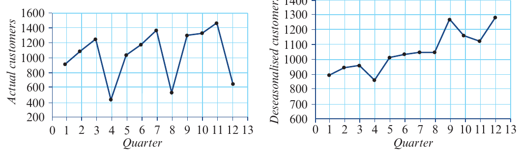
In the left graph (actual customers), the data jumps up and down dramatically due to seasonal effects. It's difficult to tell whether the business is growing or not.

In the right graph (deseasonalised customers), we can clearly see an upward trend. The business is growing steadily over time - this was hidden in the actual data by seasonal variations.

infoNote

This is why deseasonalising is so valuable: it helps us see the real trend in the data by removing the "noise" created by predictable seasonal patterns.

When to deseasonalise

Deseasonalising is particularly useful when you want to:

Identify long-term trends in your data
Compare performance across different time periods fairly
Make predictions about future performance
Fit trend lines to your data (covered in the next section)

chatImportant

Common mistakes to avoid:

Don't confuse deseasonalising (dividing) with reseasonalising (multiplying)
Don't forget to use the correct seasonal index for each time period
Don't round too early - keep full precision in intermediate calculations

bookmarkSummary

Key Points to Remember:

Seasonal indices tell us how each time period compares to the average, with an average value of 1
The sum of seasonal indices equals the number of time periods (12 for months, 4 for quarters)
Deseasonalise data by dividing: $\text{Deseasonalised} = \frac{\text{Actual}}{\text{Seasonal index}}$
Reseasonalise data by multiplying: $\text{Actual} = \text{Deseasonalised} \times \text{Seasonal index}$
Calculate seasonal indices using: $\text{Seasonal index} = \frac{\text{Value for period}}{\text{Average of all periods}}$
With multiple years of data, calculate indices for each year separately, then average them
Deseasonalising reveals the underlying trend by removing predictable seasonal patterns

For interpreting seasonal indices:

Remember that a seasonal index compares a period to the average
To find percentage above/below average, subtract 1 from the index and convert to percentage
If SI = $1.2$ , the period is $20\%$ above average
If SI = $0.8$ , the period is $20\%$ below average

For calculations:

Always check that seasonal indices sum to the number of periods
Round answers sensibly - usually to 2 or 3 decimal places for indices
When deseasonalising, divide by the seasonal index
When reseasonalising, multiply by the seasonal index
Keep track of units (dollars, customers, etc.)

Seasonal Indices (VCE SSCE General Mathematics): Revision Notes