Exponential Models and Applications Revision Notes for VCE SSCE Mathematical Methods

Exponential Models and Applications

Introduction to exponential models

Exponential functions are powerful mathematical tools that can model many real-world situations where quantities grow or decay at a constant percentage rate. In this topic, you'll learn how to apply exponential functions to various scenarios including bacterial growth, radioactive decay, population changes, and temperature changes.

infoNote

Exponential functions are among the most important mathematical models in science and everyday life. They appear in fields ranging from biology and chemistry to finance and physics. Understanding these models allows you to make predictions and analyze real-world phenomena with mathematical precision.

General exponential model

When a quantity changes exponentially over time, we can describe it using the general exponential model:

A = A_0b^t

where:

$A$ is the quantity at time $t$
$A_0$ is the initial quantity (when $t = 0$ )
$b$ is a positive constant (the base)
$t$ is time

The value of $b$ determines whether the model represents growth or decay:

When b > 1, the model represents exponential growth:

Growth of cells
Population growth
Continuously compounded interest

When b < 1, the model represents exponential decay:

Radioactive decay
Cooling of materials

chatImportant

Understanding which type of model applies to a situation helps you interpret the results and make predictions. Always check the value of $b$ first to determine if you're dealing with growth or decay before solving a problem.

Cell growth

Bacterial cells often reproduce by dividing into two new cells. This process leads to exponential growth that can be modelled mathematically.

The cell growth formula

For bacteria that divide into two cells every $T_D$ minutes:

N = N_0 2^{\frac{t}{T_D}}

where:

$N$ is the number of cells at time $t$
$N_0$ is the initial number of cells
$t$ is the time elapsed (in minutes)
$T_D$ is the generation time (the time for one cell to divide into two)

infoNote

For most bacteria that can be cultured in laboratories, generation times typically range from about 15 minutes to 1 hour. This rapid reproduction rate is why bacterial infections can spread so quickly in the body.

lightbulbExample

Worked Example: Finding Generation Time

A bacterial population increases from 5000 cells to 100,000 cells in four hours. What is the generation time?

Solution:

First, identify the known values: $N_0 = 5000$ , $N = 100\,000$ , and $t = 240$ minutes (four hours).

Substitute into the formula:

100\,000 = 5000 \times 2^{\frac{240}{T_D}}

Divide both sides by 5000:

20 = 2^{\frac{240}{T_D}}

Take $\log_2$ of both sides:

\log_2 20 = \frac{240}{T_D}

Rearrange to find $T_D$ :

T_D = \frac{240}{\log_2 20}

T_D \approx 55.53 \text{ minutes}

The generation time is approximately 55.53 minutes.

Radioactive decay

Radioactive materials naturally decay over time, with the amount of radioactive substance decreasing exponentially.

The radioactive decay formula

A = A_0 2^{-kt}

where:

$A$ is the amount of radioactive material at time $t$ (in years)
$A_0$ is the initial amount
$k$ is a positive constant that depends on the type of material
$t$ is time (in years)

The half-life of a radioactive substance is the time required for half of the material to decay. This is a key characteristic used to describe radioactive substances.

lightbulbExample

Worked Example: Calculating Half-Life

After 1000 years, a sample of radium-226 has decayed to 64.7% of its original mass. Find the half-life of radium-226.

Solution:

Use the formula $A = A_0 2^{-kt}$ with $t = 1000$ and $A = 0.647A_0$ :

0.647A_0 = A_0 2^{-1000k}

Divide by $A_0$ :

0.647 = 2^{-1000k}

Take $\log_2$ of both sides:

-1000k = \log_2 0.647

Solve for $k$ :

k = \frac{-\log_2 0.647}{1000} \approx 0.000628

To find the half-life, we need to find when $A = \frac{1}{2}A_0$ :

A_0 2^{-kt} = \frac{1}{2}A_0

2^{-kt} = \frac{1}{2}

Take $\log_2$ of both sides:

-kt = \log_2\left(\frac{1}{2}\right)

-kt = -1

t = \frac{1}{k} \approx 1591.95

The half-life of radium-226 is approximately 1592 years.

Population growth

Exponential models can sometimes be used to model population growth, although real populations often have more complex behaviour.

infoNote

While exponential models provide useful approximations for population growth, they don't account for limiting factors such as food availability, space constraints, or predation. More sophisticated models are often needed for accurate long-term predictions.

lightbulbExample

Worked Example: Kangaroo Populations

In a certain area, there are approximately ten times as many red kangaroos as grey kangaroos. The grey kangaroo population increases at 11% per annum while the red kangaroo population decreases at 5% per annum. How many years must elapse before the proportions are reversed?

Solution:

Let $G_0$ be the initial grey kangaroo population.

After $n$ years, the grey kangaroo population is:

G = G_0(1.11)^n

After $n$ years, the red kangaroo population is:

R = 10G_0(0.95)^n

When the proportions are reversed, there will be ten times as many grey kangaroos as red kangaroos:

G = 10R

Substitute the expressions:

G_0(1.11)^n = 10 \times 10G_0(0.95)^n

G_0(1.11)^n = 100G_0(0.95)^n

Divide by $G_0$ :

(1.11)^n = 100(0.95)^n

Take $\log_{10}$ of both sides:

\log_{10}((1.11)^n) = \log_{10}(100(0.95)^n)

n\log_{10} 1.11 = \log_{10} 100 + n\log_{10} 0.95

n\log_{10} 1.11 = 2 + n\log_{10} 0.95

Rearrange:

n\log_{10} 1.11 - n\log_{10} 0.95 = 2

n = \frac{2}{\log_{10} 1.11 - \log_{10} 0.95} \approx 29.6

The proportions will be reversed after approximately 30 years.

Limiting values of exponential functions

Some exponential functions approach a fixed value as time increases, rather than growing or decaying indefinitely.

Definition of limiting value

For an exponential function $f$ , if there is a real number $\ell$ such that as $x \to \infty$ , $f(x) \to \ell$ , then we say that $\ell$ is the limiting value of $f$ .

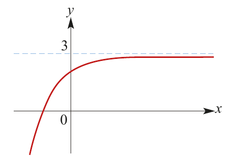
For example, consider $f(x) = 3 - 2^{-x}$ . As $x$ increases, $2^{-x}$ gets closer and closer to zero, so $f(x)$ approaches 3. The limiting value is 3.

infoNote

Limiting values are significant in many practical applications. For instance, when an object falls through a liquid, it eventually reaches a maximum speed called the terminal velocity. Similarly, when you heat or cool an object, it approaches the temperature of its surroundings.

lightbulbExample

Worked Example: Ice Pack Temperature

An ice pack is taken out of a freezer kept at -20°C. The temperature $T$ °C of the ice pack at time $t$ minutes is given by:

T = -50 \times (0.98)^t + 30

a Determine the limiting value of $T$ as $t \to \infty$ . What does this value represent?

b Determine the value of $t$ for which $T = 0$ .

c Sketch the graph of $T$ against $t$ .

d Comment on this model.

Solution:

a As $t \to \infty$ , we have $(0.98)^t \to 0$ (since $0.98 < 1$ ).

Therefore:

T \to -50 \times 0 + 30 = 30

The limiting value of $T$ is 30. This represents the outside temperature of 30°C.

b Set $T = 0$ :

-50 \times (0.98)^t + 30 = 0

-50 \times (0.98)^t = -30

(0.98)^t = 0.6

Take logarithms:

t \log 0.98 = \log 0.6

t = \frac{\log 0.6}{\log 0.98} \approx 25.285

The temperature reaches 0°C after approximately 25 minutes.

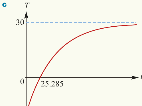
d According to the model, the ice pack approaches but never actually reaches the outside temperature. The temperature of the ice pack passes 29.9°C after about 5 hours. In practice, you would probably consider that it has reached outside temperature by this stage.

chatImportant

In theoretical models, exponential functions with limiting values approach but never quite reach their limiting value. However, in practical applications, we often consider the limit to be "reached" when the function gets sufficiently close to it.

Determining exponential rules

Sometimes you need to find the rule for an exponential function when given specific information about points on the curve.

lightbulbExample

Worked Example: Finding the Exponential Rule

The points $(1, 6)$ and $(5, 96)$ lie on the curve $y = a \times b^x$ , where $a > 0$ and $b > 0$ . Find the values of $a$ and $b$ .

Solution:

Since the points lie on the curve, we can write:

a \times b^1 = 6 \quad \text{...(1)}

a \times b^5 = 96 \quad \text{...(2)}

Divide equation (2) by equation (1):

\frac{a \times b^5}{a \times b^1} = \frac{96}{6}

b^4 = 16

b = 16^{\frac{1}{4}} = 2

Substitute $b = 2$ into equation (1):

a \times 2 = 6

a = 3

Therefore, a = 3 and b = 2.

Using a calculator to find exponential rules

CAS calculators can solve these problems efficiently by solving simultaneous equations.

infoNote

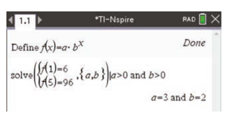
The calculator confirms that $a = 3$ and $b = 2$ . Using technology to verify your algebraic solutions is a good practice, especially for more complex problems.

Fitting data to exponential models

When you have real-world data, you can use exponential regression to find an exponential model that fits the data.

Example: modelling weight increase

Consider Somu, an orangutan born at the Eastern Plains Zoo. The table shows Somu's weight for the first 6 months:

Months, $m$	$0$	$1$	$2$	$3$	$4$	$5$	$6$
Weight (kg), $w$	$1.65$	$1.7$	$2.2$	$3.0$	$3.7$	$4.2$	$4.8$

These data values can be plotted alongside an exponential function to see how well it fits.

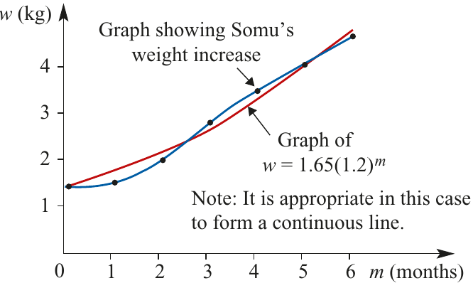
The exponential model $w = 1.65(1.2)^m$ approximates the actual weight gain. This model describes a growth rate of 20% per month for the first 6 months.

infoNote

It is appropriate to draw a continuous line through the data points, even though weight is only measured at specific times, because the orangutan's weight changes continuously. This is an important distinction when modeling real-world phenomena.

Using exponential regression

A CAS calculator can perform exponential regression to find the best-fitting exponential model for a set of data.

For Somu's weight data, exponential regression gives:

w = 1.55(1.22)^m

This model can be used to predict future weight gains for orangutan births at the zoo. The slight difference from the manual model ( $1.65(1.2)^m$ ) shows that regression finds the statistically best fit to the data.

chatImportant

When using exponential models to make predictions, be cautious about extrapolating too far beyond the original data range. The model may not remain accurate over extended periods, especially for biological systems where growth patterns change over time.

bookmarkSummary

Key Points to Remember:

Exponential models have the form $A = A_0b^t$ , where b > 1 represents growth and b < 1 represents decay
Cell growth uses the formula $N = N_0 2^{\frac{t}{T_D}}$ , where $T_D$ is the generation time
Radioactive decay uses the formula $A = A_0 2^{-kt}$ , where the half-life can be found using $t = \frac{1}{k}$
The limiting value of an exponential function is the value that the function approaches as time increases indefinitely
You can determine exponential rules by using given points to create and solve simultaneous equations
Exponential regression allows you to fit real-world data to an exponential model for prediction and analysis

Exponential Models and Applications (VCE SSCE Mathematical Methods): Revision Notes