Graphing Logarithmic Functions (VCE SSCE Mathematical Methods): Revision Notes
Graphing Logarithmic Functions
Understanding logarithmic graphs
Logarithmic functions have a distinctive curved shape that is quite different from other functions you may have studied. The most important thing to understand is that logarithmic functions are the inverse of exponential functions, which means their graphs are reflections of each other across the line .
When we plot an exponential function such as alongside its inverse logarithmic function , we can see this inverse relationship clearly. The two curves mirror each other across the diagonal line .
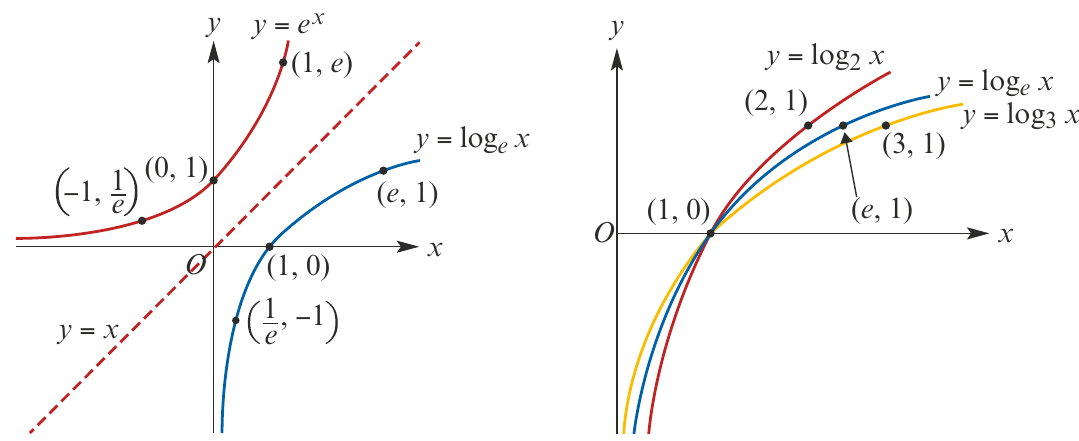
The reflection property across is a fundamental characteristic of all inverse function pairs. This visual relationship helps us understand why exponential and logarithmic functions "undo" each other.
Key features of
For any logarithm with base (meaning is positive and not equal to 1), the graph of has several important characteristics that you need to know:
Three Key Points on Every Logarithmic Graph:
- The point always lies on the curve
- The point is always on the curve (this is the x-intercept)
- The point is always on the curve
These three points are extremely useful when sketching logarithmic graphs because they give you a framework to work with.
Domain and range:
- The domain is (all positive real numbers)
- The range is (all real numbers)
This means you can only take the logarithm of positive numbers, but the output can be any real number, positive or negative.
Vertical asymptote:
- The y-axis (the line ) is a vertical asymptote
This means the graph approaches the y-axis but never touches or crosses it. As gets closer to zero from the positive side, the function value decreases without bound (approaches negative infinity for ).
Properties based on the base value
The base of the logarithm determines whether the function is increasing or decreasing:
When : The logarithmic function is strictly increasing. This means as increases, also increases. The function is also one-to-one, meaning each -value corresponds to exactly one -value, and vice versa.
When : The logarithmic function is strictly decreasing. This means as increases, decreases. The function is still one-to-one.
In both cases, the one-to-one property is what makes logarithmic functions invertible. This property is essential for solving logarithmic equations.
Transformations of logarithmic graphs
When we apply transformations to the basic logarithmic function (where ), we need to understand how the graph changes.
For graphs of the form where :
- The vertical asymptote is at
- The domain is
- The x-intercept is at
These rules help us quickly determine the key features of transformed logarithmic functions.
Worked example: dilation transformation
Worked Example: Sketching a Dilated Logarithmic Function
Sketch the graph of .
Solution:
To create this graph, we start with the basic natural logarithm function and apply two transformations:
Step 1: Apply a dilation of factor 3 from the x-axis (this stretches the graph vertically by a factor of 3)
Step 2: Apply a dilation of factor from the y-axis (this compresses the graph horizontally by a factor of 2)
The transformation mapping is
This means we transform the key points:
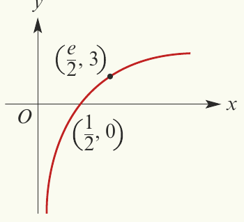
Result: The graph maintains the vertical asymptote at (the y-axis) and still has domain and range .
Worked example: translation transformations
Worked Example: Sketching Translated Logarithmic Functions
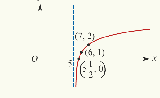
Sketch the graph and state the implied domain of:
a)
This graph is obtained from by applying two translations:
- 5 units in the positive x-direction (shift right)
- 1 unit in the positive y-direction (shift up)
The transformation mapping is
Key points transform as follows:
Finding the asymptote:
The vertical asymptote shifts from to
Finding the x-intercept:
When :
Domain:
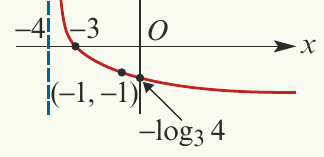
b)
This graph is obtained from by applying:
- A reflection in the x-axis (the negative sign flips the graph)
- A translation of 4 units in the negative x-direction (shift left)
The transformation mapping is
Key points transform as follows:
Finding the asymptote:
The vertical asymptote shifts from to
Finding the y-intercept:
When :
Domain:
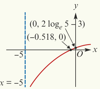
Worked example: combined transformations
Worked Example: Sketching with Multiple Transformations
Sketch the graph of and state the implied domain.
Solution:
This transformation involves:
- A dilation of factor 2 from the x-axis (vertical stretch)
- A translation of 5 units in the negative x-direction (shift left)
- A translation of 3 units in the negative y-direction (shift down)
Finding the asymptote:
The vertical asymptote is at
Finding the intercepts:
When :
When :
Domain:
Converting between different logarithmic bases
Sometimes we need to convert a logarithm from one base to another. This is particularly useful when comparing logarithmic functions with different bases or when using a calculator.
Base Conversion Formula:
To change the base of from to (where and ), we use:
Deriving this formula:
Starting with , we know that by the definition of logarithms.
Taking of both sides:
Since , we get the formula above.
Graphical interpretation:
The graph of can be obtained from the graph of by applying a dilation of factor from the x-axis.
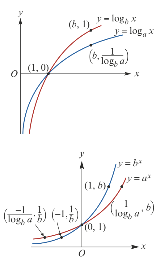
This means the graph is stretched or compressed vertically depending on the relationship between the two bases. The point remains fixed (since for any base), but other points scale vertically.
Remember!
Key Points to Remember:
- Key points: Every logarithmic graph passes through , , and
- Domain restriction: You can only take logarithms of positive numbers, so the domain is always for the basic function
- Vertical asymptote: The basic logarithmic function has a vertical asymptote at (the y-axis)
- Transformations shift the asymptote: For , the asymptote moves to
- Base conversion: Use to convert between bases