Graphs of Exponential Functions Revision Notes for VCE SSCE Mathematical Methods

Graphs of Exponential Functions

Introduction

Exponential functions create distinctive curved graphs that differ significantly from linear or polynomial functions. Understanding their shape and properties is essential for working with growth and decay models in mathematics and real-world applications.

There are two main types of exponential graphs to explore, determined by the value of the base.

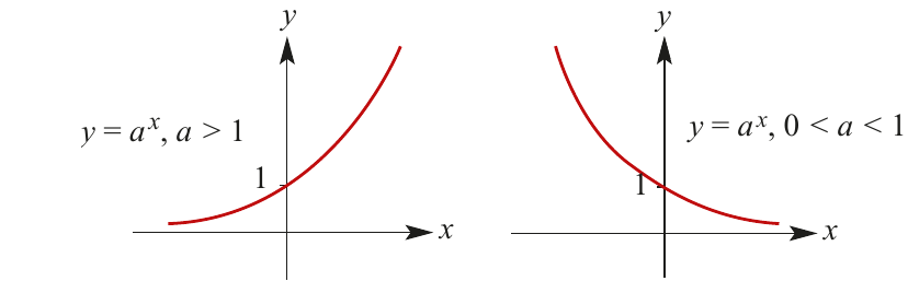
Exponential growth: graphs of $y = a^x$ when $a > 1$

When the base of an exponential function is greater than 1, the graph displays exponential growth.

lightbulbExample

Worked Example: Sketching $y = 2^x$

Let's plot the graph of $y = 2^x$ by creating a table of values for $-3 \leq x \leq 3$ .

$x$	$-3$	$-2$	$-1$	$0$	$1$	$2$	$3$
$y = 2^x$	$\frac{1}{8}$	$\frac{1}{4}$	$\frac{1}{2}$	$1$	$2$	$4$	$8$

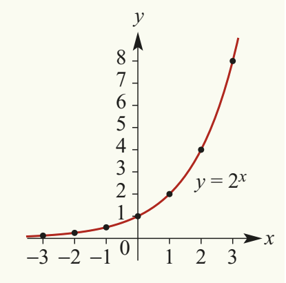
Notice how the y-values become very small (but positive) for negative x-values, and they increase rapidly as x becomes positive.

Key properties of exponential growth graphs

When examining graphs of the form $y = a^x$ where $a > 1$ , several important features emerge:

Asymptotic behavior: As x takes increasingly large negative values, the y-values approach zero but never actually reach it. The graph gets closer and closer to the x-axis from above, making the x-axis a horizontal asymptote.

We write this as: As $x \to -\infty$ , $y \to 0^+$

infoNote

This notation means "as x approaches negative infinity, y approaches 0 from the positive side."

Increasing nature: As x-values increase, the y-values also increase. The function is always increasing across its entire domain.

Y-intercept: The graph always crosses the y-axis at the point (0, 1). This makes sense because $a^0 = 1$ for any positive base $a$ .

Domain and range:

The domain is $\mathbb{R}$ (all real numbers) - you can input any real value for x
The range is $\mathbb{R}^+$ (positive real numbers) - the output is always positive

lightbulbExample

Worked Example: Sketching $y = 10^x$

Let's examine another exponential growth function with a larger base. For $y = 10^x$ with $-1 \leq x \leq 1$ :

Table

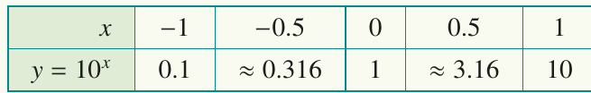
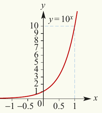
Observations:

The x-axis remains an asymptote
The y-intercept is still at $(0, 1)$
As x increases, y increases
For any given x-value, $y = 10^x$ grows more rapidly than $y = 2^x$

chatImportant

Larger bases produce steeper exponential growth. This is a key principle when comparing different exponential functions: the bigger the base (when $a > 1$ ), the faster the function increases.

Relationship between different bases

All exponential functions with bases greater than 1 are related through horizontal dilations (stretches or compressions from the y-axis). For example, the graph of $y = 10^x$ can be obtained from $y = 2^x$ by applying a specific dilation factor from the y-axis.

Exponential decay: graphs of $y = a^x$ when $0 < a < 1$

When the base lies between 0 and 1, the exponential function displays decay rather than growth.

lightbulbExample

Worked Example: Sketching $y = \left(\frac{1}{2}\right)^x$

Let's plot $y = \left(\frac{1}{2}\right)^x$ for $-3 \leq x \leq 3$ . Note that this can also be written as $y = 2^{-x}$ .

$x$	$-3$	$-2$	$-1$	$0$	$1$	$2$	$3$
$y = \left(\frac{1}{2}\right)^x$	$8$	$4$	$2$	$1$	$\frac{1}{2}$	$\frac{1}{4}$	$\frac{1}{8}$

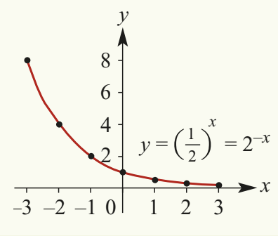
This graph slopes downward from left to right, opposite to the behavior when $a > 1$ .

Key properties of exponential decay graphs

For graphs of the form $y = a^x$ where $0 < a < 1$ :

Asymptotic behavior: The x-axis is still a horizontal asymptote, but now the graph approaches it from above as x increases (rather than decreases).

We write: As $x \to \infty$ , $y \to 0^+$

Decreasing nature: As x-values increase, the y-values decrease toward zero.

Y-intercept: The graph still passes through (0, 1).

Domain and range:

Domain: $\mathbb{R}$ (all real numbers)
Range: $\mathbb{R}^+$ (positive real numbers only)

General properties of exponential graphs

Comparing both types of exponential functions reveals their similarities and differences.

infoNote

Common features for all exponential functions $y = a^x$ (regardless of whether $a > 1$ or $0 < a < 1$ ):

The x-axis (line $y = 0$ ) serves as a horizontal asymptote
The y-intercept is always at $(0, 1)$
The y-values are always positive - the graph never crosses or touches the x-axis
There is no x-intercept
The domain is $\mathbb{R}$
The range is $\mathbb{R}^+$

Reflection relationship

An important connection exists between exponential growth and decay functions. For any exponential function, we can express $y = a^x$ as $y = b^{-x}$ where $b = \frac{1}{a}$ .

For example, if $f(x) = 2^x$ and $g(x) = \left(\frac{1}{2}\right)^x$ , then:

g(x) = \left(\frac{1}{2}\right)^x = (2^{-1})^x = 2^{-x} = f(-x)

chatImportant

This means the graph of $y = \left(\frac{1}{2}\right)^x$ is the reflection of $y = 2^x$ in the y-axis, and vice versa.

Using technology to analyze exponential graphs

Graphing calculators provide powerful tools for investigating exponential functions in detail.

Finding specific coordinate values

lightbulbExample

Worked Example: Finding y when x = 2.1

For the function $y = 2^x$ , find the value of y when $x = 2.1$ .

Using a graphing calculator:

Plot the graph of $y = 2^x$
Use the trace or evaluate function to find the point where $x = 2.1$

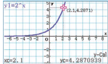
The result shows that when $x = 2.1$ , $y = 4.287$ (correct to three decimal places).

Finding intersection points

lightbulbExample

Worked Example: Finding x when y = 9

For the function $y = 2^x$ , find the value of x when $y = 9$ .

Approach:

Plot both $y = 2^x$ and the horizontal line $y = 9$ on the same screen
Find their intersection point

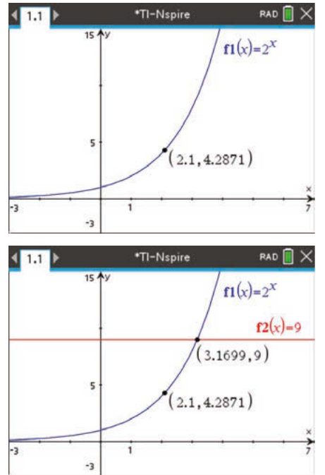
The calculator shows that when $y = 9$ , $x = 3.170$ (correct to three decimal places).

This technique is particularly useful for solving exponential equations graphically.

Transformations of exponential graphs

Exponential functions can be transformed using the same techniques applied to other function types: translations, dilations, and reflections.

Vertical translations

Adding a constant to an exponential function shifts the graph vertically and moves the asymptote.

lightbulbExample

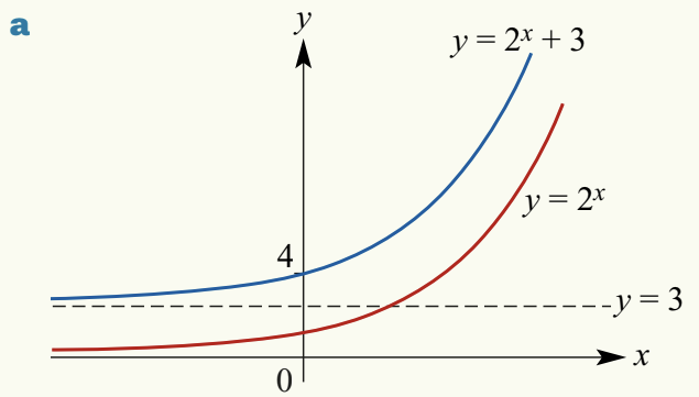
Worked Example: Vertical Translation

Compare $f(x) = 2^x$ and $g(x) = 2^x + 3$

The graph of $y = 2^x + 3$ is obtained by translating $y = 2^x$ upward by 3 units.

Key features of $g(x) = 2^x + 3$ :

Asymptote: $y = 3$ (shifted from $y = 0$ )
Y-intercept: $(0, 4)$ since $2^0 + 3 = 4$
Range: $(3, \infty)$

Vertical dilations

Multiplying an exponential function by a constant stretches or compresses it vertically.

lightbulbExample

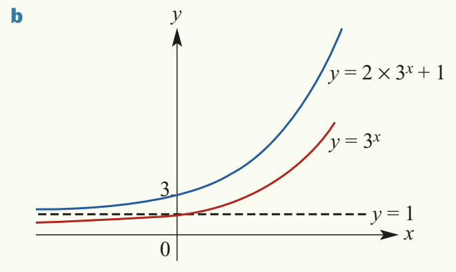
Worked Example: Vertical Dilation and Translation

Compare $f(x) = 3^x$ and $g(x) = 2 \times 3^x + 1$

The graph of $y = 2 \times 3^x + 1$ involves two transformations:

Vertical dilation by factor 2 from the x-axis
Vertical translation upward by 1 unit

Key features of $g(x) = 2 \times 3^x + 1$ :

Asymptote: $y = 1$ (the translation affects the asymptote)
Y-intercept: $(0, 3)$ since $2 \times 3^0 + 1 = 3$
Range: $(1, \infty)$

Reflections in the x-axis

Multiplying by $-1$ reflects the graph in the x-axis and reverses the range.

lightbulbExample

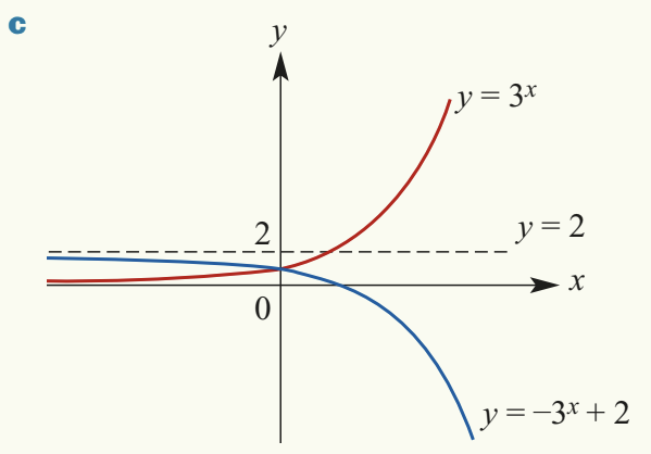
Worked Example: Reflection in the x-axis

Compare $f(x) = 3^x$ and $g(x) = -3^x + 2$

The graph of $y = -3^x + 2$ is obtained through:

Reflection in the x-axis (the negative sign)
Vertical translation upward by 2 units

Key features of $g(x) = -3^x + 2$ :

Asymptote: $y = 2$ (shifted from $y = 0$ )
Y-intercept: $(0, 1)$ since $-3^0 + 2 = 1$
Range: $(-\infty, 2)$ (note the range is now bounded above instead of below)

Horizontal dilations

Modifying the exponent creates horizontal compressions or stretches.

lightbulbExample

Worked Example: Horizontal Dilation

Compare $y = 3^x$ and $y = 3^{2x}$

The graph of $y = 3^{2x}$ is obtained from $y = 3^x$ by a horizontal dilation (compression) by factor $\frac{1}{2}$ from the y-axis.

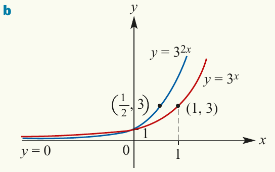
Both graphs share:

The same asymptote: $y = 0$
The same y-intercept: $(0, 1)$

However, $y = 3^{2x}$ increases more rapidly because the exponent is doubled.

Combined transformations

Multiple transformations can be applied in sequence.

lightbulbExample

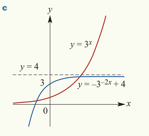
Worked Example: Multiple Transformations

Sketch $y = -3^{-2x} + 4$

Starting from $y = 3^x$ , apply these transformations in order:

Horizontal dilation by factor $\frac{1}{2}$ from the y-axis (giving $y = 3^{2x}$ )
Reflection in the y-axis (giving $y = 3^{-2x}$ )
Reflection in the x-axis (giving $y = -3^{-2x}$ )
Vertical translation upward by 4 units (giving $y = -3^{-2x} + 4$ )

Key features:

Asymptote: $y = 4$
Range: $(-\infty, 4)$

chatImportant

The order of transformations matters when combining multiple changes to a function. Always apply transformations in the correct sequence to obtain the desired result.

bookmarkSummary

Key Points to Remember:

All exponential graphs of the form $y = a^x$ pass through the point (0, 1)
For $a > 1$ , the graph shows exponential growth (increasing from left to right)
For $0 < a < 1$ , the graph shows exponential decay (decreasing from left to right)
The x-axis is always a horizontal asymptote; exponential functions are always positive
Larger bases (when $a > 1$ ) produce steeper growth curves
The graph of $y = \left(\frac{1}{a}\right)^x$ is the reflection in the y-axis of the graph $y = a^x$
Transformations affect the asymptote: vertical translations shift it, but horizontal transformations don't

Graphs of Exponential Functions (VCE SSCE Mathematical Methods): Revision Notes