Instantaneous Rate of Change Revision Notes for VCE SSCE Mathematical Methods

Instantaneous Rate of Change

Introduction

In previous sections, we explored the average rate of change of a function over an interval. We discovered that for non-linear functions, the average rate of change varies depending on which interval we choose. Now we'll investigate a more precise concept: the instantaneous rate of change at a specific point.

The instantaneous rate of change tells us how quickly a function is changing at a particular moment, rather than over an interval. This is fundamental in understanding motion, growth patterns, and many other real-world phenomena.

infoNote

Think of instantaneous rate of change like checking a car's speedometer at a specific moment - it tells you exactly how fast you're going right now, not your average speed over a trip.

Understanding tangent lines

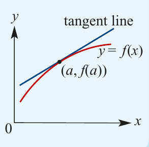
A tangent line to a curve at a point is a straight line that has the same slope as the curve at that exact point. Imagine zooming in very close to a point on a curve - the curve starts to look more and more like a straight line. This "local" straight line is what we call the tangent.

To understand this better, let's consider a specific example using the parabola $y = x^2$ and find the tangent line at point $P(1, 1)$ .

The secant line approach

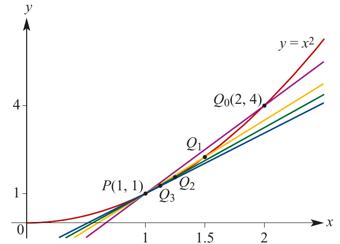
We start by drawing a secant line - a line passing through two points on the curve. Let's begin with secant $PQ_0$ passing through $P(1, 1)$ and $Q_0(2, 4)$ .

The gradient of $PQ_0$ is:

\frac{4 - 1}{2 - 1} = 3

So the equation of secant $PQ_0$ is $y = 3x - 2$ .

chatImportant

The Key Idea: We'll create more points $Q_1, Q_2, Q_3, \ldots$ on the curve that get progressively closer to point $P$ . As these points get closer, the secant lines will approach the tangent line.

We calculate each point's $x$ -coordinate by finding the midpoint between $P$ and the previous $Q$ point:

$x$ -coordinate of $Q_1 = \frac{1}{2}(1 + 2) = \frac{3}{2}$
$x$ -coordinate of $Q_2 = \frac{1}{2}(1 + \frac{3}{2}) = \frac{5}{4}$
$x$ -coordinate of $Q_3 = \frac{1}{2}(1 + \frac{5}{4}) = \frac{9}{8}$

Observing the pattern

As we draw secant lines through $P$ and each of these points, something remarkable happens. Here's a table showing the gradient and equation of each secant:

Step	Point on curve	Secant	Gradient	Equation of secant
0	$Q_0(2, 4)$	$PQ_0$	$3$	$y = 3x - 2$
1	$Q_1(\frac{3}{2}, \frac{9}{4})$	$PQ_1$	$\frac{5}{2}$	$y = \frac{5}{2}x - \frac{3}{2}$
2	$Q_2(\frac{5}{4}, \frac{25}{16})$	$PQ_2$	$\frac{9}{4}$	$y = \frac{9}{4}x - \frac{5}{4}$
3	$Q_3(\frac{9}{8}, \frac{81}{64})$	$PQ_3$	$\frac{17}{8}$	$y = \frac{17}{8}x - \frac{9}{8}$
$n$	$Q_n(1 + 2^{-n}, (1 + 2^{-n})^2)$	$PQ_n$	$2 + 2^{-n}$	$y = (2 + 2^{-n})x - (1 + 2^{-n})$

The sequence of gradients is: $3, \frac{5}{2}, \frac{9}{4}, \frac{17}{8}, \ldots, 2 + \frac{1}{2^n}, \ldots$

infoNote

Observing the Convergence:

Notice what happens to the general gradient $2 + \frac{1}{2^n}$ . As $n$ increases towards infinity, $\frac{1}{2^n}$ approaches zero, so the gradient approaches $2$ .

This tells us that the secant lines are getting closer and closer to a line with gradient $2$ and equation $y = 2x - 1$ . This is our tangent line!

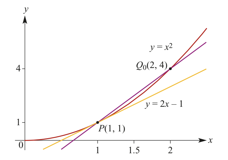
The gradient of the tangent line represents the instantaneous rate of change of $y$ with respect to $x$ at point $P$ .

Estimating instantaneous rate of change

In this course, we approximate the instantaneous rate of change by calculating the gradient of a secant line through two very close points.

lightbulbExample

Worked Example: Estimating Instantaneous Rate of Change

Estimate the instantaneous rate of change of $y$ with respect to $x$ at point $P(2, 9)$ on the curve $y = x^3 + 1$ by considering the secant $PQ$ , where $Q = (2.01, (2.01)^3 + 1)$ .

Solution:

Gradient of $PQ = \frac{(2.01)^3 + 1 - 9}{2.01 - 2}$

Therefore, the instantaneous rate of change at $P(2, 9)$ is approximately 12.06.

infoNote

Improving Accuracy:

For even better accuracy, we could choose points closer together, such as $P(2, 9)$ and $Q(2.001, (2.001)^3 + 1)$ . This would give us $12.006$ . The closer the points, the better our approximation. The true instantaneous rate of change is actually $12$ .

lightbulbExample

Worked Example: Plant Growth

The graph shows the area covered by a spreading plant, measured in square centimetres over time in weeks.

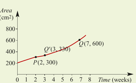
Part a: Find the gradient of secant $PQ$ .

Solution:

Gradient of $PQ = \frac{600 - 300}{7 - 2}$

The average rate of change of area from $t = 2$ to $t = 7$ is $60$ cm² per week.

Part b: Point $Q'$ has coordinates $(3, 330)$ . Find the average rate of change of area with respect to time for interval $[2, 3]$ , and use this to estimate the instantaneous rate of change at $t = 2$ .

Solution:

Gradient of $PQ' = \frac{330 - 300}{3 - 2}$

Therefore, the gradient at $P$ is approximately $30$ .

The instantaneous rate of change of the plant's area with respect to time when $t = 2$ is approximately $30$ cm² per week.

lightbulbExample

Worked Example: Exponential Function

Consider the curve $y = 2^x$ .

Part a: Using the secant through points where $x = 3$ and $x = 3.1$ , estimate the instantaneous rate of change of $y$ with respect to $x$ where $x = 3$ .

Solution:

When $x = 3$ : $y = 2^3 = 8$

When $x = 3.1$ : $y = 2^{3.1} = 8.5742$ (to four decimal places)

\text{Gradient} = \frac{8.5742 - 8}{3.1 - 3} = \frac{0.5742}{0.1} = 5.742

The instantaneous rate of change at $x = 3$ is approximately 5.742.

Part b: Repeat using points where $x = 3$ and $x = 3.001$ .

Solution:

When $x = 3.001$ : $y = 2^{3.001} = 8.005547$

\text{Gradient} = \frac{8.005547 - 8}{3.001 - 3} = \frac{0.005547}{0.001} = 5.547

The closer points give us 5.547, which is nearer to the true value of $5.5452$ (to four decimal places).

Using graphing technology

Graphing calculators provide another method for estimating instantaneous rate of change. By zooming in on a curve near a point, the curve appears increasingly linear, allowing us to estimate the gradient.

infoNote

Technology Approach:

For example, consider the function $y = 0.5x^3 - 2x + 1$ at point $(0, 1)$ .

Starting with secant $RS$ where $R = (-0.75, 2.2891)$ and $S = (0.25, 0.5078)$ :

\text{Gradient of } RS = \frac{0.5078 - 2.2891}{0.25 - (-0.75)} = -1.7813

Using a closer point $R_1 = (-0.25, 1.4922)$ :

\text{Gradient of } R_1S = \frac{0.5078 - 1.4922}{0.25 - (-0.25)} = -1.9688

By zooming in further and using points $A = (-0.1, 1.1995)$ and $B = (0.1, 0.8005)$ :

\text{Gradient} = \frac{0.8005 - 1.1995}{0.1 - (-0.1)} = \frac{-0.399}{0.2} \approx -2

Therefore, the gradient at $(0, 1)$ is approximately -2.

Key definition

chatImportant

Definition: Instantaneous Rate of Change

For a function $y = f(x)$ , the instantaneous rate of change of $y$ with respect to $x$ at point $(a, f(a))$ is the gradient of the tangent line to the graph of $y = f(x)$ at that point.

bookmarkSummary

Key Points to Remember:

The instantaneous rate of change at a point is the gradient of the tangent line at that point
We can approximate the instantaneous rate of change by finding the gradient of a secant through two nearby points
The closer the points are together, the better our approximation
Secant lines approach the tangent line as the second point gets closer to the first point
In practical applications, the instantaneous rate of change tells us the rate of change at a specific moment in time or at a specific value

Instantaneous Rate of Change (VCE SSCE Mathematical Methods): Revision Notes