Aggregate Demand and Economic Activity Revision Notes for AQA A-Level Economics

Aggregate Demand and Economic Activity

What is economic activity?

Economic activity refers to the overall level of production and consumption taking place within an economy. It encompasses the creation of goods and services, alongside the utilisation of productive resources such as labour, capital, and other factors of production needed to generate output.

When we discuss economic activity, we're looking at how busy the economy is in terms of producing things people want and need, and how much employment is generated in the process.

infoNote

The buying and selling of goods and services represents one key aspect of economic activity. Shopping centres, like the one shown above, are hubs where consumer spending takes place, contributing directly to the level of economic activity in the economy.

How aggregate demand influences economic activity

Understanding the relationship between aggregate demand and economic activity is crucial for analysing macroeconomic performance. Changes in aggregate demand directly affect the level of real output produced in the economy, which in turn influences employment levels.

The link between aggregate demand and real output

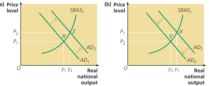
We can use aggregate demand and aggregate supply (AD/AS) diagrams to illustrate how shifts in aggregate demand affect the level of real output. Whilst these diagrams don't directly show employment levels, there's a clear connection: when real output increases, firms generally need to employ more workers to produce the additional goods and services. Conversely, when real output falls, less labour is required to produce the smaller quantity of goods and services being made.

chatImportant

Understanding the Two Key Scenarios:

The diagrams above demonstrate two important scenarios:

Panel (a) - Expansionary effect: When aggregate demand increases (shifting rightward from $AD_1$ to $AD_2$ ), the equilibrium moves from point X to point Z. This results in:

An increase in the price level (from $P_1$ to $P_2$ )
An increase in real national output (from $y_1$ to $y_2$ )
Higher employment, as firms need more workers to meet increased demand

Panel (b) - Contractionary effect: When aggregate demand decreases (shifting leftward from $AD_2$ to $AD_1$ ), the equilibrium moves from point X to point V. This causes:

A decrease in the price level (from $P_1$ to $P_2$ )
A decrease in real national output (from $y_1$ to $y_2$ )
Lower employment, as firms need fewer workers due to reduced demand

Important factors affecting the size of output changes

Two key points determine how much real output changes when aggregate demand shifts:

The size of the shift in aggregate demand - A larger shift in the AD curve produces a greater change in real output
The steepness of the aggregate supply curve - The extent to which real output changes also depends on how steep the AS curve is

Aggregate demand and the national income multiplier

Understanding the multiplier concept

The national income multiplier measures the relationship between an initial change in a component of aggregate demand (such as government spending or private investment) and the resulting, typically larger, change in the level of national income.

Here's how it works: imagine the government increases spending by £10 billion on infrastructure projects whilst keeping tax revenue unchanged. This creates a budget deficit that injects £10 billion of new spending into the circular flow of income. This initial spending increases people's incomes. Assuming that most people in the economy save only a small portion of any income increase and spend the rest, the £10 billion generates multiple rounds of further spending.

infoNote

Each round of spending creates progressively smaller increases in income, until the next round becomes so tiny it can be ignored. When we add up all these successive stages of income generation, the total increase in income becomes a multiple of the initial £10 billion spending increase - hence the term "multiplier theory".

The multiplier in action

Let's say the multiplier has a value of 2.5. An increase in a component of aggregate demand, such as government spending of £10 billion, would cause national income to eventually increase by £25 billion.

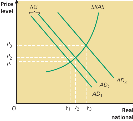
The diagram above illustrates this process on an AD/AS diagram. An initial increase in government spending ( $\Delta G$ ) shifts the AD curve from $AD_1$ to $AD_2$ . This triggers the multiplier process, leading to a further increase in aggregate demand to $AD_3$ . When the government spending multiplier equals 2.5, the eventual increase in aggregate demand is two and a half times larger than the initial increase in government spending.

Calculating the multiplier

The multiplier relationship can be expressed mathematically:

$\text{multiplier} = \frac{\text{change in national income}}{\text{initial change in government spending}}$

Or using symbols:

$\text{multiplier} = \frac{\Delta Y}{\Delta G}$

Where:

$\Delta Y$ represents the change in national income
$\Delta G$ represents the change in government spending

To calculate the size of the multiplier, we need to know both the change in aggregate demand and the resulting change in national income.

lightbulbExample

Worked Example: Calculating the Multiplier

In an economy, nominal national income is £2,000 billion in 2021. Government spending increases by £10 billion. This causes nominal national income to increase to £2,050 billion in 2022.

Solution:

The increase in government spending of £10 billion causes nominal national income to increase by £50 billion between 2021 and 2022.

The size of the multiplier in terms of growth in nominal national income is therefore:

$\text{multiplier} = \frac{£50 \text{ billion}}{£10 \text{ billion}} = 5$

This represents quite a large multiplier.

Different types of multipliers

Whilst we've focused on the government spending multiplier, there are actually several types of multipliers operating within the economy:

Government spending multiplier - relates to changes in public expenditure
Tax multiplier - shows the effect of changes in taxation
Export multiplier - measures the impact of changes in export spending
Import multiplier - shows the effect of changes in imports
Investment multiplier - relates to changes in private sector investment

Together, the government spending and tax multipliers are known as fiscal policy multipliers. Similarly, the export and import multipliers are called foreign trade multipliers.

chatImportant

The Multiplier Can Work in Reverse!

It's important to note that the multiplier process can work in reverse. Rather than increasing national income, it can reduce it. This happens when government spending, consumption, investment, or exports fall, or when taxation or imports increase. This is because taxation and imports represent withdrawals from the circular flow of income, rather than injections.

The tax and import multipliers are always negative, meaning that an increase in taxes or imports causes national income to fall, whilst a decrease in taxes or imports causes national income to rise.

Regional multipliers

Besides national multipliers, regional multipliers can also be important. A regional multiplier measures the relationship between an initial change in aggregate demand and the resulting change in regional income.

For example, if the central government pays a subsidy to people in Cornwall, the recipients spend the extra income they receive. However, most of this spending may occur on goods and services produced in other parts of the UK, or even on imports. Consequently, the regional multiplier, which reflects extra local spending within Cornwall, is likely to be very small.

infoNote

Study tip: Don't confuse the multiplier with the accelerator. They're easy to mix up because both concepts examine the relationship between AD (especially the investment component in the case of the accelerator) and national income. The key difference lies in understanding which variable changes to cause a change in the other variable.

The marginal propensities to consume and save

Before explaining the formula for calculating the multiplier's size, we need to understand two key concepts: the marginal propensity to consume and the marginal propensity to save.

Marginal propensity to consume (MPC)

The marginal propensity to consume represents the fraction of any increase in income that people plan to spend on consumption of domestically produced goods and services.

For example, if people on average plan to spend 90p out of every £1 increase in income on consumption, the MPC equals 0.9.

Marginal propensity to save (MPS)

The marginal propensity to save represents the fraction of any increase in income that people plan to save rather than spend.

If the MPC is 0.9, then the MPS must be 0.1, because together they must add up to 1. When people receive extra income, they either spend it or save it - there's no third option.

chatImportant

Critical Relationship:

$\text{MPC} + \text{MPS} = 1$

This fundamental relationship means that any income received must be either consumed or saved - there is no third alternative.

How the MPC affects the multiplier

The size of the multiplier depends heavily on the marginal propensity to consume:

High MPC = Large multiplier

When marginal propensities to consume are high, most new income gets spent on consumption at each stage of the multiplier process, with only a small amount leaking into saving. In this situation, multipliers are relatively large. An initial increase in government spending or private investment has a substantial multiplier effect because each round of spending remains large.

Low MPC = Small multiplier

Conversely, a low MPC (and therefore high MPS) produces the opposite effect: the eventual growth in income resulting from the multiplier process isn't much larger than the initial increase in aggregate demand. When saving and other leakages from the circular flow of income are quite high, multipliers tend to be small, not significantly different from 1.

The multiplier formula

The formula for calculating the value of the multiplier is:

$k = \frac{1}{1 - \text{MPC}}$

or equivalently:

$k = \frac{1}{\text{MPS}}$

Where:

$k$ represents the multiplier
$\text{MPC}$ represents the marginal propensity to consume
$\text{MPS}$ represents the marginal propensity to save

lightbulbExample

Worked Example: Calculating Multiplier Values

Calculate the size of the multiplier when, in a closed economy with no exports or imports, the marginal propensity to consume (MPC) is:

(a) 0.6

Solution:

When the MPC is 0.6, the multiplier equals:

$k = \frac{1}{1 - 0.6} = \frac{1}{0.4} = 2.5$

(b) 0.4

Solution:

When the MPC is 0.4, the multiplier equals:

$k = \frac{1}{1 - 0.4} = \frac{1}{0.6} = 1.67$

Key Observation: Notice how a higher MPC produces a larger multiplier value.

The multiplier as a dynamic process

The multiplier process doesn't happen instantaneously - it takes place over time. Think of it like ripples spreading over a pond after a stone has been thrown into the water. However, whilst ripples in a pond last only a few seconds, the ripples spreading through the economy following a change in aggregate demand can last for months or even years.

infoNote

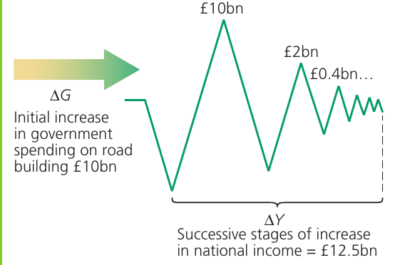
The diagram above illustrates the dynamic nature of the multiplier process, showing how an initial injection of government spending generates successive waves of income increases that diminish over time.

How the multiplier process unfolds over time

Let's work through a detailed example to understand the stages:

Stage 1 - Initial injection

The £10 billion of extra government spending is received as income by building workers who construct new roads. Assuming the marginal propensity to consume (MPC) is 0.2 throughout the economy (meaning people plan to consume 20p out of every £1 increase in income), workers spend 20% of their extra income on consumption. This means that at each stage of the multiplier process, 80% of any extra income leaks out of the circular flow through saving, taxation, and spending on imports, whilst only 20% is spent on consumption.

Stage 2 - First round of respending

£2 billion of the £10 billion income is spent on consumer goods and services, with the remaining £8 billion leaking into savings, tax payments, and spending on imports.

Stage 3 - Second round of respending

Consumer goods sector employees spend £0.4 billion (20% of the £2 billion they received at stage 2) on further consumption.

Subsequent stages

Further rounds of income generation continue, with each successive stage being 0.2 times the size of the previous stage. Each wave of spending becomes progressively smaller because a large portion of income leaks into savings, taxation, and imports at each stage.

The final outcome

Assuming nothing else changes in the time taken for the process to work through the economy, the eventual increase in income ( $\Delta Y$ ) resulting from the initial injection of government spending is the sum of all the stages of income generation.

infoNote

Key insight: The assumption of quite a small MPC of 0.2 is realistic for the UK and many other developed economies, as a large fraction of any increase in income leaks out of the circular flow through taxation and spending on imports, in addition to saving.

In this example with an MPC of 0.2, the eventual increase in income ( $\Delta Y$ ) is larger than $\Delta G$ (the initial government spending increase), but the multiplier is quite small (1.25) because of the large size of leakages at each stage of the multiplier process.

Nominal national income, real national income and the size of the multiplier

It's crucial to understand the relationship between nominal and real measures of national income:

$\text{nominal national income} = \text{real national income} \times \text{average price level}$

Or in shorthand:

$Y = P \cdot y$

Where:

$Y$ represents nominal national income
$P$ represents the price level
$y$ represents real national income

Why this distinction matters for the multiplier

The size of the multiplier depends on whether we're measuring the nominal national income multiplier or the real national income multiplier.

In the earlier example, the multiplier size was 1.25, but this represented the nominal national income multiplier. Provided the short-run aggregate supply (SRAS) curve slopes upward, as shown in typical AD/AS diagrams, the size of the multiplier measured in real terms is always smaller than the nominal national income multiplier.

This occurs because part of the multiplier effect translates into a rising price level rather than increased real output. The growth of real income becomes restricted to the distance between $y_1$ and $y_2$ on the horizontal axis, with the price level rising from $P_1$ to $P_2$ .

The extreme case of a vertical SRAS curve

chatImportant

When the Multiplier Effect Only Creates Inflation

If the SRAS curve were vertical rather than upward sloping, the size of the multiplier measured in real income terms would be zero. In this situation, the multiplier effect resulting from an increase in government spending would lead solely to inflation, without any increase in real output.

This demonstrates an important principle: when the economy is operating at or near full capacity, the multiplier effect mainly causes inflation rather than real output growth.

bookmarkSummary

Key Points to Remember:

Economic activity encompasses the production and consumption of goods and services, along with the employment needed to generate output.
Changes in aggregate demand directly affect real output and employment - when AD increases, output and employment typically rise; when AD falls, output and employment typically decline.
The multiplier effect means that an initial change in spending (such as government spending) leads to a larger overall change in national income through successive rounds of spending.
The marginal propensity to consume (MPC) is the fraction of extra income that people spend, whilst the marginal propensity to save (MPS) is the fraction they save - together they always equal 1.
A higher MPC creates a larger multiplier because more income gets respent at each stage, whilst a lower MPC creates a smaller multiplier due to greater leakages.
The multiplier formula is $k = \frac{1}{1 - \text{MPC}}$ or $k = \frac{1}{\text{MPS}}$ , allowing you to calculate the multiplier's value when you know the spending and saving propensities.
The multiplier process takes time - it works through the economy in successive waves of spending that become progressively smaller.
The real multiplier is smaller than the nominal multiplier when the SRAS curve slopes upward, because part of the effect translates into higher prices rather than increased real output.

Aggregate Demand and Economic Activity (AQA A-Level Economics): Revision Notes