Determination of Equilibrium Market Prices (AQA A-Level Economics): Revision Notes
Determination of Equilibrium Market Prices
Introduction to market equilibrium
In a competitive market, the interaction between demand and supply determines the price at which goods and services are bought and sold. This section explores how the market reaches a balance point called equilibrium, where the plans of consumers and producers align perfectly.
To understand this concept, we'll use the tomato market as our main example. In this market, numerous consumers wish to buy tomatoes at various prices, whilst many farmers and firms wish to sell tomatoes. The question is: at what price do these opposing forces find balance?
The concept of market equilibrium is fundamental to understanding how prices are determined in competitive markets. By examining a simple example like tomatoes, we can see these economic principles at work in everyday situations.
Understanding equilibrium and disequilibrium
Before examining how prices are determined, we need to understand two fundamental concepts that describe market conditions.
Equilibrium refers to a point where market forces are balanced, creating a state of rest. When a market is in equilibrium, there is no tendency for change because the opposing forces of supply and demand are equal. Think of it like a set of perfectly balanced scales - neither side tips up or down.
Disequilibrium, by contrast, describes a situation where these market forces are not in balance. When a market is in disequilibrium, there are pressures pushing for change, just like unbalanced scales that tip to one side.
Key Definitions:
-
Market equilibrium occurs at a specific price where the quantity consumers wish to purchase exactly matches the quantity producers wish to sell. This is the point where the demand curve intersects (crosses) the supply curve on a diagram. At this price, both buyers and sellers can fulfil their plans.
-
Market disequilibrium exists at any price other than the equilibrium price. In this situation, either:
- Consumers wish to buy more than producers wish to sell (excess demand), or
- Producers wish to sell more than consumers wish to buy (excess supply)
When disequilibrium occurs, the price will not remain stable - market forces will push it towards the equilibrium level.
The interaction of demand and supply
Let's examine how market demand and supply work together to determine price and quantity in a competitive market.
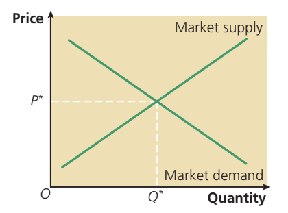
The market demand curve shows the total quantity of a good that all consumers in the market plan to purchase at different price levels during a particular time period. This curve slopes downward from left to right, reflecting the inverse relationship between price and quantity demanded. When prices are high, fewer consumers are willing or able to buy tomatoes; when prices fall, more consumers enter the market or existing buyers purchase more.
The market supply curve shows the total quantity of a good that all producers in the market wish to supply at different price levels during the same time period. This curve slopes upward, demonstrating the positive relationship between price and quantity supplied. Higher prices make production more profitable, encouraging firms to supply greater quantities.
Equilibrium price (P*) is determined at the exact point where these two curves intersect. At this price, the quantity demanded by consumers equals the quantity supplied by producers. The market 'clears' - meaning all the goods that firms wish to sell find buyers, and all consumers who want to purchase at this price can do so.
Equilibrium quantity (Q*) is the amount of the good that changes hands at the equilibrium price. This represents the actual volume of transactions that take place in the market.
The asterisk symbol () is commonly used in economics to denote equilibrium values. So P means "equilibrium price" and Q* means "equilibrium quantity". These represent the price and quantity where the market naturally settles when left to its own devices.
Market disequilibrium: excess supply and excess demand
Most of the time, markets are not at their equilibrium price. When prices differ from equilibrium, either excess supply or excess demand occurs, triggering automatic market adjustments.
Excess supply
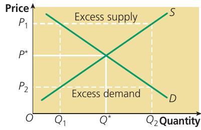
Excess supply (also called a surplus) occurs when the market price sits above the equilibrium level. At this higher price, firms wish to sell more than consumers wish to buy.
For example, imagine tomato producers set their price at P₁, which is above the equilibrium price P*. At this price:
- Producers would like to supply quantity Q₂
- Consumers only wish to purchase quantity Q₁
- The difference (Q₂ - Q₁) represents excess supply or unsold stock
Producers cannot sell all the tomatoes they wish to at price P₁. Some tomatoes remain unsold, creating unwanted inventory. To eliminate this surplus, producers reduce their prices. As the price falls, two things happen simultaneously: consumers buy more (moving along the demand curve) and some producers reduce their output (moving along the supply curve). This adjustment continues until the price reaches P*, where excess supply disappears.
Excess demand
Excess demand (also called a shortage) occurs when the market price is below equilibrium. At this lower price, consumers wish to buy more than firms wish to supply.
For instance, if the price of tomatoes is P₂ (below equilibrium):
- Consumers would like to buy quantity Q₂
- Producers only wish to supply quantity Q₁
- The difference (Q₂ - Q₁) represents excess demand or unfulfilled demand
Not all consumers can purchase the tomatoes they want at price P₂. This shortage creates upward pressure on price. Some disappointed buyers may offer to pay more, whilst producers realise they can charge higher prices. As the price rises, quantity demanded decreases and quantity supplied increases until equilibrium is restored at P*.
The market adjustment mechanism
The process described above is called the market adjustment mechanism. It's helpful to think about markets having two 'sides':
- The short side of the market consists of the economic agents (buyers or sellers) who can always fulfil their plans
- The long side of the market contains those who cannot fulfil their plans at the current price
When price is above equilibrium (P₁), households and consumers are on the short side - they can buy exactly the quantity of tomatoes they wish (Q₁). Tomato producers are on the long side - they want to sell Q₂ but can only sell Q₁. The difference represents unsold stock.
When price is below equilibrium (P₂), the situation reverses. Producers are on the short side and can sell all they produce (Q₁), whilst consumers are on the long side, unable to buy as much as they want. The difference represents unmet demand.
This adjustment mechanism operates automatically in free markets, with no need for government intervention. Prices act as signals, guiding resources towards their most valued uses.
The market adjustment process:
- Excess supply → Price falls → Movement along curves → Equilibrium restored
- Excess demand → Price rises → Movement along curves → Equilibrium restored
Summary of disequilibrium conditions
Market disequilibrium occurs when:
- Planned demand is less than planned supply, causing the price to fall, or
- Planned demand is greater than planned supply, causing the price to rise
Market equilibrium occurs when:
- Planned demand equals planned supply, and the price remains stable
How supply shifts disturb market equilibrium
Once a market reaches equilibrium, it remains there until an external event causes either the supply curve or the demand curve to shift position. Let's first examine what happens when supply changes.
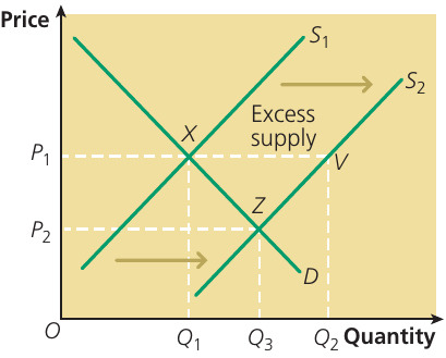
Consider the tomato market where equilibrium initially exists at point X, with price P₁ and quantity Q₁. The market remains stable at this point until something changes the conditions of supply.
Suppose a bumper harvest occurs due to favourable weather conditions. This causes the supply curve to shift rightward from S₁ to S₂, indicating that producers can and will supply more tomatoes at every price level.
However, at the original equilibrium price P₁, the market is no longer in equilibrium. Looking at the diagram:
- At price P₁, producers now wish to supply quantity Q₃ (point V on the new supply curve S₂)
- Consumers still only wish to purchase quantity Q₁ (point X on the demand curve)
- The difference between Q₃ and Q₁ represents excess supply
To eliminate this surplus stock, tomato producers must reduce their prices. The market price falls from P₁ towards P₂. As the price decreases:
- Consumers move along their demand curve, purchasing more tomatoes
- Producers move along their new supply curve S₂, reducing the quantity they supply
The market settles at a new equilibrium (point Z) where the new supply curve S₂ intersects the unchanged demand curve D. At this point:
- The new equilibrium price is P₂ (lower than before)
- The new equilibrium quantity is Q₂ (higher than before)
- Planned supply once again equals planned demand
Key Principle:
When supply increases (rightward shift), equilibrium price falls and equilibrium quantity rises, assuming demand remains constant.
This makes intuitive sense - when more of a good is available in the market, its price typically decreases, but the total amount bought and sold increases.
How demand shifts disturb market equilibrium
Just as supply shifts create disequilibrium, changes in demand also disturb market equilibrium and trigger price adjustments.
Let's examine what happens in the tomato market when consumer demand increases. Tomatoes are usually considered a normal good - a product for which demand increases as consumer incomes rise. When household incomes grow, people tend to buy more tomatoes (and other goods).
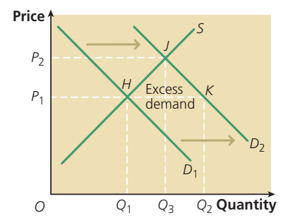
Initially, the market is in equilibrium where demand curve D₁ intersects the supply curve S at price P₁ and quantity Q₁. Consumers and producers can both fulfil their plans at this point.
Now suppose consumer incomes increase significantly. This shifts the market demand curve rightward from D₁ to D₂, showing that at every price level, consumers now wish to purchase more tomatoes than before.
At the original price P₁, equilibrium no longer exists:
- Consumers now wish to buy a much larger quantity (shown at point K on demand curve D₂)
- Producers are only willing to supply quantity Q₁ (point H on the supply curve)
- The difference between these quantities (distance H to K) represents excess demand
Consumers cannot buy all the tomatoes they want at price P₁. Competition among buyers drives the price upward. As the price increases to P₂:
- The quantity of tomatoes purchased and sold rises from Q₁ to Q₂
- There is movement along the supply curve from point H to point J, representing an extension of supply as producers respond to higher prices
- The excess demand is eliminated
The market establishes a new equilibrium at point J where:
- The new equilibrium price is P₂ (higher than before)
- The new equilibrium quantity is Q₂ (greater than before)
- The market once again clears, with planned demand equalling planned supply
Key Principle:
When demand increases (rightward shift), both equilibrium price and equilibrium quantity rise, assuming supply remains constant.
This reflects the reality that when consumers want more of a product (perhaps due to rising incomes or changing preferences), both the price and the quantity traded in the market increase.
Calculating equilibrium price: a worked example
We can determine equilibrium price and quantity not only through diagrams but also by using supply and demand schedules - tables showing the quantities demanded and supplied at different prices.
Worked Example: Finding Equilibrium in the Chocolate Bar Market
| Price per bar (£) | Quantity of bars demanded per week | Quantity of bars supplied per week |
|---|---|---|
| 0.75 | 180 | 240 |
| 0.70 | 200 | 200 |
| 0.65 | 220 | 160 |
| 0.60 | 240 | 120 |
This table shows the demand and supply schedules for chocolate bars in a particular market.
Step 1: Identify the equilibrium price
To find the equilibrium price, we need to identify the price at which the quantity demanded equals the quantity supplied. Examining the table:
- At £0.75: Quantity demanded (180) < Quantity supplied (240) = Excess supply of 60 bars
- At £0.70: Quantity demanded (200) = Quantity supplied (200) = EQUILIBRIUM
- At £0.65: Quantity demanded (220) > Quantity supplied (160) = Excess demand of 60 bars
- At £0.60: Quantity demanded (240) > Quantity supplied (120) = Excess demand of 120 bars
The equilibrium price is £0.70 per bar, with an equilibrium quantity of 200 bars per week.
Step 2: Analyse the effect of a supply increase
Now suppose that due to a fall in the price of cocoa beans (a key input), the supply of chocolate bars rises by 60 bars at all prices. We can construct a new supply schedule:
- At £0.75: New supply = 240 + 60 = 300 bars
- At £0.70: New supply = 200 + 60 = 260 bars
- At £0.65: New supply = 160 + 60 = 220 bars
- At £0.60: New supply = 120 + 60 = 180 bars
Looking for the new equilibrium (where quantity demanded equals new quantity supplied):
At £0.65: Quantity demanded (220) = New quantity supplied (220) = NEW EQUILIBRIUM
Step 3: State the outcome
Therefore, the increase in supply causes:
- Equilibrium price to fall from £0.70 to £0.65
- Equilibrium quantity to rise from 200 to 220 bars per week
This confirms our earlier analysis: an increase in supply (rightward shift of the supply curve) leads to a lower equilibrium price and a higher equilibrium quantity.
Exam tips
Understanding equilibrium and disequilibrium is fundamental to economics. These concepts help explain why markets move from one state to another and form the foundation for more advanced topics you'll encounter later.
Key points to remember for exams:
-
Always distinguish between a shift of a curve (caused by factors other than price, moving the entire curve left or right) and movement along a curve (caused by price changes, moving from one point to another on the same curve)
-
When analysing market changes, follow this approach:
- Identify whether supply or demand has changed
- Determine which direction the curve shifts
- Identify the initial disequilibrium created
- Explain the market adjustment mechanism
- State the new equilibrium price and quantity
-
In your later studies, you'll encounter other types of equilibrium including profit-maximising equilibrium, equilibrium wage rate, equilibrium national income, and balance of payments equilibrium. The core concept remains the same - a balance between opposing forces.
-
Price acts as a signalling mechanism in markets. When prices rise or fall, they signal to producers and consumers to adjust their behaviour, guiding resources towards their most valued uses.
-
Remember that in competitive markets with many buyers and sellers, the adjustment to equilibrium happens automatically through the price mechanism, without need for central coordination.
Remember!
Key Points to Remember:
-
Market equilibrium occurs where the demand curve intersects the supply curve, determining both equilibrium price and equilibrium quantity
-
Excess supply (surplus) exists when price is above equilibrium, causing unsold stock and downward pressure on price
-
Excess demand (shortage) exists when price is below equilibrium, causing unmet demand and upward pressure on price
-
Supply increases (rightward shifts) lead to lower prices and higher quantities at the new equilibrium
-
Demand increases (rightward shifts) lead to higher prices and higher quantities at the new equilibrium
-
Markets automatically adjust towards equilibrium through the price mechanism - excess supply causes prices to fall, whilst excess demand causes prices to rise