Supply of Goods and Services (AQA A-Level Economics): Revision Notes
Supply of Goods and Services
Introduction to market supply
When economists discuss supply in a market context, they are referring to market supply. This represents the total amount of a good or service that all producers in a given market are willing and able to offer for sale at various price levels during a specific time period.
Market supply differs from individual supply in an important way. While individual supply shows what one particular firm wishes to sell, market supply aggregates the intentions of all firms operating in that market. Think of it as adding up what every producer plans to supply at each possible price point.
The key difference between individual and market supply is simple: market supply = the sum of all individual firm supplies at each price level. If Firm A supplies 100 units at $10 and Firm B supplies 150 units at $10, the market supply at $10 is 250 units.
The relationship between price and quantity supplied is straightforward: market supply represents the sum total of what all producers in a market plan to offer at different price levels. This collective intention forms the basis for understanding how markets function.
Understanding the supply curve
Characteristics of supply curves
A supply curve provides a visual representation of the relationship between the price of a good and the quantity that producers are willing to supply. The curve displays an upward slope, moving from left to right, which reflects a fundamental principle in economics.
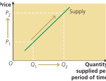
When we examine a supply curve, we see that as prices increase from P₁ to P₂, the quantity supplied rises from Q₁ to Q₂. This positive relationship between price and quantity supplied is a defining feature of market supply.
It's important to note that the horizontal axis shows "Quantity supplied per period of time" rather than just "Quantity". This reminds us that supply is measured over a specific timeframe, whether that's per day, per week, or per year.
Why supply curves slope upward
The upward slope of supply curves stems from the profit-maximising behaviour of firms. Producers in a market economy aim to maximise their profits, and this objective directly influences their supply decisions.
Profit represents the difference between the total revenue a firm earns from selling its goods or services and the total costs incurred in producing them. Total revenue refers to all the money a firm receives from selling its complete output.
The Profit Motive Drives Supply
Higher prices → Higher potential profit → Greater incentive to produce → More supply
This fundamental relationship explains why supply curves slope upward. Firms respond to price signals by adjusting their production levels to maximise profits.
When prices are low, firms find it less attractive to produce goods because the potential profit is limited. However, as prices rise, producing and selling becomes more profitable. This creates an incentive for existing firms to expand their production. Additionally, higher prices may attract entirely new firms to enter the market, further increasing overall supply.
Consider the costs involved in production. When a firm produces more units of a good, the cost of making each additional unit generally increases. This happens because firms eventually face constraints on their resources and production capacity. Therefore, firms will only choose to supply more if the price rises sufficiently to compensate for these higher production costs.
Exam tip: Movements along the curve
Remember that when the price of a good changes, we observe a movement along the supply curve, not a shift of the entire curve. This is a crucial distinction. A price change causes producers to move to a different point on the existing supply curve, supplying either more (at higher prices) or less (at lower prices). The curve itself doesn't move.
Shifts in the supply curve
While price changes cause movements along a supply curve, other factors can cause the entire curve to shift to a new position. We call these factors the conditions of supply.
A condition of supply is any determinant of supply other than the product's own price. These factors influence how much producers are willing to supply at every possible price level. When one or more conditions of supply change, assuming the ceteris paribus (all other things being equal) assumption no longer holds, the supply curve shifts.
Critical Distinction: Movement vs Shift
- Movement along the curve = caused by a change in the good's own price
- Shift of the curve = caused by a change in conditions of supply (anything other than the good's price)
Confusing these two concepts is one of the most common mistakes in economics exams!
Increase and decrease in supply
When the supply curve shifts rightward, we call this an increase in supply. This means producers are willing to supply more of the good at every price level than before.
Conversely, a leftward shift represents a decrease in supply, indicating that producers will supply less at every price level.
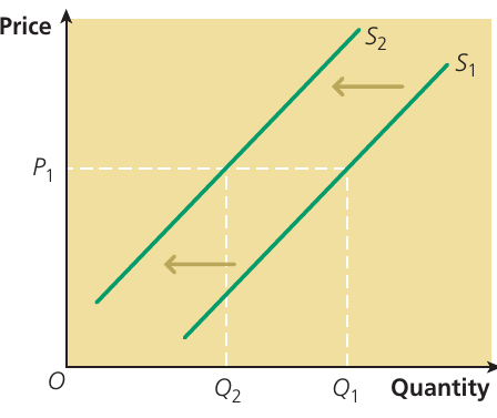
The diagram above illustrates a leftward shift in supply from S₁ to S₂. Notice that at price P₁, the quantity supplied falls from Q₁ to Q₂. This decrease in supply means that at the same price, less is now available in the market.
Memory Aid: "Right is More, Left is Less"
- Rightward shift = increase in supply = more available at every price
- Leftward shift = decrease in supply = less available at every price
Think of the horizontal axis representing quantity: moving right means more, moving left means less!
The conditions of supply
Several key factors determine the position of the supply curve. Understanding these conditions helps explain why supply might increase or decrease:
Production costs
Changes in the costs of production significantly impact supply decisions. These costs include:
Wage costs: Labour represents a major expense for most firms. If wages rise, production becomes more expensive, making it less profitable to produce the same quantity. This causes supply to decrease (shift left). Conversely, if wage costs fall, supply increases.
Raw material costs: The price of inputs needed for production affects supply. For example, if steel prices rise, car manufacturers face higher costs, reducing their willingness to supply at current prices.
Energy costs: Many production processes require substantial energy. Increases in electricity or fuel prices raise production costs, shifting supply leftward.
Borrowing costs: Firms often borrow money to finance production or expansion. If interest rates rise, borrowing becomes more expensive, discouraging production and decreasing supply.
The Cost-Supply Relationship
The relationship between production costs and supply is inverse:
- When production costs ↑ → Supply ↓ (shifts left)
- When production costs ↓ → Supply ↑ (shifts right)
This applies to ALL types of production costs: wages, materials, energy, and borrowing costs.
Technical progress
Technological improvements can significantly boost supply. When firms adopt better production methods or more efficient machinery, they can produce more output using the same resources, or the same output at lower cost. This reduction in production costs shifts the supply curve rightward, increasing supply at all price levels.
Worked Example: Technology and Supply
Consider a bakery that traditionally kneads bread by hand:
- Before: 10 workers can produce 200 loaves per day
- After new machinery: Same 10 workers can now produce 400 loaves per day
The technological improvement means:
- Production costs per loaf have fallen
- The bakery can supply more at every price level
- Supply curve shifts rightward
Taxes on firms
Governments may impose various taxes on producers, such as VAT, excise duties, or business rates. From a firm's perspective, these taxes function similarly to an increase in production costs. The firm must now pay additional money to the government for each unit produced or sold, making production less profitable.
An increase in taxes imposed on firms shifts the supply curve leftward (upwards), representing a decrease in supply. For instance, when the price is P₁ and the government introduces a tax, the quantity firms are prepared to supply falls from Q₁ to Q₂.
Government subsidies
A subsidy is a payment from the government to firms, effectively reducing their production costs. Subsidies have the opposite effect to taxes – they shift the supply curve rightward, increasing supply at all price levels.
When firms receive subsidies, production becomes more profitable even at lower prices, encouraging them to supply more. This makes the good more available in the market.
Tax vs Subsidy: Mirror Effects
- Taxes: Increase costs → Decrease supply → Shift LEFT
- Subsidies: Decrease costs → Increase supply → Shift RIGHT
Both are tools for government intervention in markets, but they work in opposite directions!
Government intervention and supply
Expenditure taxes and their effects
Governments use expenditure taxes as a way to generate revenue, but these taxes significantly impact market supply. There are two main types of expenditure taxes that affect supply differently:
Ad valorem taxes
An ad valorem tax is levied as a percentage of a good's price. Value Added Tax (VAT) is the most common example in the UK, typically charged at 20% on the price of most goods and services.
When an ad valorem tax is imposed, the supply curve shifts leftward, but in a specific way. Because the tax is a percentage of the price, the tax amount increases as the price increases. This means the vertical distance between the old and new supply curves gets larger at higher prices, making the new supply curve steeper than the original.
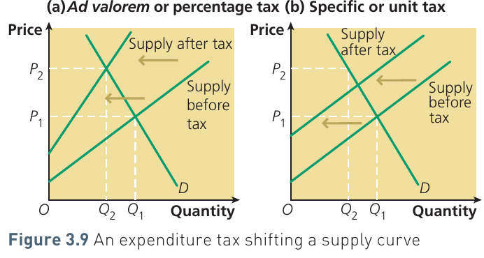
The diagram shows both ad valorem and specific tax effects. In panel (a), notice how the new supply curve after the ad valorem tax has a steeper slope than the original. At a price of £1, if the tax rate is 20%, the government collects 20p in tax revenue per unit sold. However, if the price is £2, the government collects 40p per unit.
Worked Example: Ad Valorem Tax Calculation
A product sells for £50, and the government introduces a 20% ad valorem tax.
Step 1: Calculate the tax amount Tax = 20% × £50 = £10
Step 2: Determine the new price New price = £50 + £10 = £60
Step 3: Compare with different price If the original price were £100: Tax = 20% × £100 = £20 New price = £120
Key insight: The absolute tax amount increases with price (£10 vs £20), which is why the supply curve becomes steeper.
Specific (unit) taxes
A specific tax (also called a unit tax) is a fixed amount charged per unit of a good sold, regardless of the price. For example, excise duty on tobacco is levied as a set amount per packet, not as a percentage of the price.
When a specific tax is imposed, the supply curve shifts vertically upward by the exact amount of the tax. Unlike ad valorem taxes, the vertical distance between the old and new supply curves remains constant at all price levels. This means the two supply curves are parallel to each other, as shown in panel (b) of the diagram.
Distinguishing Tax Types
Ad valorem tax:
- Percentage of price
- Tax amount varies with price
- Supply curves NOT parallel
- Example: 20% VAT
Specific tax:
- Fixed amount per unit
- Tax amount constant regardless of price
- Supply curves ARE parallel
- Example: £2.50 per packet of cigarettes
Tax effects on market outcomes
Both types of taxes effectively pass on costs to consumers by increasing the price of goods. Firms must charge higher prices to maintain profitability after paying the tax. The final price consumers pay rises from P₁ to P₂, while the quantity traded in the market falls from Q₁ to Q₂.
From an economic perspective, expenditure taxes provide examples of indirect taxes. Although firms pay the tax directly to the government, consumers ultimately bear much of the burden through higher prices.
Subsidies and supply
Government subsidies work in the opposite direction to taxes. When the government provides subsidies to producers, it effectively reduces their costs of production.
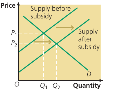
A subsidy causes the supply curve to shift rightward (downward), indicating an increase in supply. After receiving a subsidy, firms can afford to supply more of the good at each price level, or supply the same amount at a lower price.
Specific subsidies
In the case of a specific subsidy (a fixed amount per unit), the sum of money the government pays to firms remains the same for each unit produced, regardless of the good's price. This causes the supply curve to shift rightward by a constant amount at all price levels.
Like specific taxes, this results in the two supply curves (before and after subsidy) being parallel to each other. The vertical distance between them equals the subsidy amount per unit.
The market effects are clear: the equilibrium price falls from P₁ to P₂, making the good more affordable for consumers, while the quantity traded increases from Q₁ to Q₂.
Ad valorem subsidies
If a subsidy were calculated as a percentage of the price (ad valorem subsidy), the subsidy amount would vary with the good's price. In this case, the supply curve shift would not be parallel, similar to how ad valorem taxes work.
Exam Tip: Tax and Subsidy Analysis
When analysing taxes and subsidies, always remember:
- Taxes shift supply leftward (or upward) – decreasing supply
- Subsidies shift supply rightward (or downward) – increasing supply
- The type of tax/subsidy (ad valorem vs specific) determines whether supply curves are parallel or not
- Both taxes and subsidies affect equilibrium price and quantity in the market
A useful framework: State the intervention → Identify the shift direction → Explain the effect on price and quantity → Consider who benefits/loses
Price elasticity of supply
While we understand that supply responds to price changes, the extent of this response varies between different goods. Price elasticity of supply measures how responsive the quantity supplied is to changes in a good's price.
The formula
We calculate price elasticity of supply using the following formula:
This formula gives us a numerical value that indicates the degree of supply responsiveness. The calculation is similar in structure to price elasticity of demand, but focuses on supply-side responses.
Understanding the PES Formula
The formula compares:
- Numerator: How much quantity supplied changes (in %)
- Denominator: How much price changes (in %)
If quantity supplied changes by a larger percentage than price, supply is elastic (PES > 1). If quantity supplied changes by a smaller percentage than price, supply is inelastic (PES < 1).
Interpreting elasticity values
Understanding what different elasticity values mean is crucial for analysis:
Elastic supply: When the supply curve intersects the price axis (the vertical axis), the curve is elastic at all points along it. As you move up the curve from point to point, elasticity falls but always remains greater than 1. This means quantity supplied responds more than proportionately to price changes.
Inelastic supply: If the supply curve intersects the quantity axis (the horizontal axis), it is inelastic at all points. Moving up the curve, elasticity rises towards unity (1) but never reaches it. Here, quantity supplied responds less than proportionately to price changes.
Unit elastic supply: A supply curve passing through the origin (where both axes meet) has an elasticity equal to unity (+1) at all points. This means quantity supplied changes by exactly the same percentage as price.
Worked Example: Calculating PES
A product's price increases from £20 to £25, and quantity supplied rises from 1,000 to 1,400 units.
Step 1: Calculate percentage change in price
Step 2: Calculate percentage change in quantity supplied
Step 3: Apply the PES formula
Interpretation: PES = 1.6 means supply is elastic. A 1% increase in price leads to a 1.6% increase in quantity supplied.
Important distinction: Slope vs elasticity
A common mistake is confusing the slope of a supply curve with its elasticity. These are not the same thing!
Don't Confuse Slope with Elasticity!
- Slope measures the steepness of the line (change in price ÷ change in quantity)
- Elasticity measures the proportional responsiveness (% change in quantity ÷ % change in price)
Even though upward-sloping straight-line supply curves may look similar, they can have very different elasticities depending on where they intersect the axes. The slope tells us about the steepness of the line, while elasticity tells us about the proportional responsiveness of quantity to price.
Remember: A steep curve doesn't necessarily mean inelastic supply, and a flat curve doesn't necessarily mean elastic supply!
Exam tip: Using PES in analysis
Price elasticity of supply is particularly useful when:
- Analysing how markets respond to sudden changes in demand
- Evaluating the likely effects of government taxes or subsidies
- Understanding why some markets adjust quickly to price changes while others don't
- Assessing the impact of production constraints on market equilibrium
Key Points to Remember:
• Market supply represents the total quantity all firms in a market plan to sell at different prices over a specific time period.
• Supply curves slope upward because higher prices make production more profitable, encouraging firms to supply more and attracting new firms to the market.
• Changes in conditions of supply (production costs, technology, taxes, or subsidies) shift the entire supply curve, while price changes cause movements along the curve.
• Taxes on firms decrease supply (shift left/upward) while subsidies increase supply (shift right/downward), with different effects depending on whether they're ad valorem or specific.
• Price elasticity of supply measures supply responsiveness to price changes, calculated as the percentage change in quantity supplied divided by the percentage change in price – don't confuse slope with elasticity!
Memory Aid - CWET-TS for Conditions of Supply:
- Costs of production
- Wages
- Energy costs
- Technical progress
- Taxes
- Subsidies