Costs of Producton (AQA A-Level Economics): Revision Notes
Costs of Production
Understanding costs of production is essential in economics. This note explains how firms calculate and analyse their production costs, focusing on the different types of costs and how they behave as output changes.
Short-run costs
The difference between short-run and long-run costs
In economics, the short run is defined as the time period in which at least one factor of production remains fixed. During this period, firms face two types of costs:
- Fixed costs: costs that do not change with the level of output produced in the short run
- Variable costs: costs that change as the level of output changes
Consider a factory example: the factory's rent remains the same whether it produces 100 units or 1,000 units (fixed cost), but the cost of raw materials increases with production (variable cost). This illustrates the fundamental difference between these two cost types.
The relationship between these costs can be expressed mathematically:
Total cost = Total fixed cost + Total variable cost
Or using abbreviations:
Similarly, for average costs:
Average total cost = Average fixed cost + Average variable cost
Or:
In contrast, long-run costs are always variable. This is because in the long run, all factors of production can be changed. A firm can expand or reduce its factory size, change locations, or adjust all aspects of production. Therefore, the distinction between fixed and variable costs only applies to the short run.
The difference between fixed and variable costs
Fixed costs represent the expenses a firm must pay for the fixed factors of production, regardless of output level. These costs remain unchanged in the short run and typically include:
- Rent on land and buildings
- Maintenance costs of premises
- Initial cost of acquiring buildings and factory space
- Interest payments on loans
Variable costs change directly with the level of output produced. As production increases or decreases, variable costs rise or fall accordingly. Common examples include:
- Wages paid to workers
- Cost of raw materials
- Energy costs for production
- Delivery and distribution costs
In the long run, when all factors of production can be varied, all costs become variable costs. The firm can adjust its scale of operations, relocate, or completely restructure its production methods. The fixed-variable cost distinction is a short-run phenomenon only.
The difference between total cost, average variable cost and marginal cost
When analysing production costs, firms need to understand three key concepts:
Total cost (TC) represents all costs incurred when producing a particular quantity of output. At any output level, this equals the sum of total fixed costs and total variable costs.
Average variable cost (AVC) is calculated by dividing total variable cost by the quantity of output produced. This tells us the variable cost per unit of output:
Marginal cost (MC) represents the additional cost incurred when producing one more unit of output. This is a crucial concept for decision-making, as firms need to know how much extra it costs to increase production by one unit.
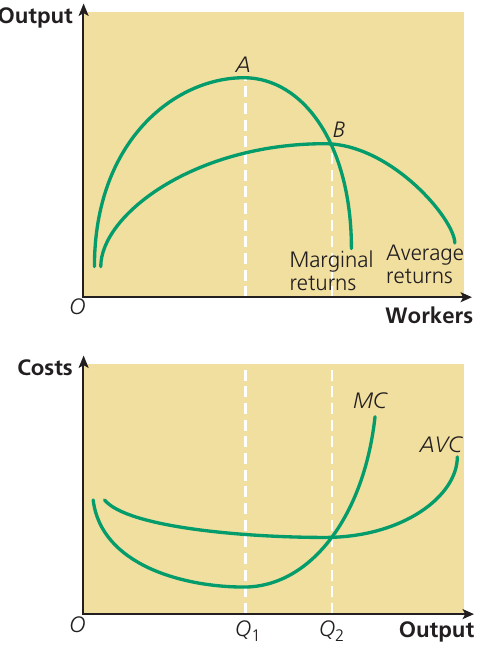
The diagram above illustrates the relationship between production and costs. The top panel shows how output changes as more workers are employed, demonstrating diminishing marginal returns. The bottom panel shows the corresponding cost curves, with marginal cost (MC) and average variable cost (AVC) both forming U-shaped curves.
The short-run average fixed cost (AFC) curve
Fixed costs must be paid regardless of production levels, but their impact per unit of output changes as production varies. Average fixed cost (AFC) measures the fixed cost per unit of output:
Or:
Worked Example: Spreading of Overheads
Consider a car manufacturing company with annual overheads of £1 million:
- If the plant produces only one car per year, the AFC per car is £1,000,000
- With two cars, the AFC falls to £500,000 per car
- With three cars, it drops to £333,333 per car
- As production continues to increase, AFC keeps falling
This demonstrates how fixed costs are distributed across more units as output rises.
This phenomenon is known as the spreading of overheads. As output increases, fixed costs are spread across more units, causing the average fixed cost per unit to fall continuously.
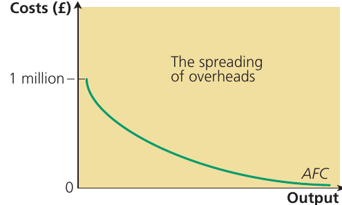
The AFC curve always slopes downwards from left to right. As output increases, average fixed costs approach zero but never actually reach it. At very high levels of output, the AFC becomes negligible, though fixed costs are still being paid.
The short-run average total cost (ATC) curve
The average total cost (ATC) curve shows the total cost per unit of output at different production levels. It is calculated as:
Or:
This can also be expressed as:
The ATC curve is derived by adding the AFC and AVC curves together at each level of output. Initially, as production increases from zero, average costs tend to fall. However, beyond a certain point, average costs begin to rise, creating the characteristic U-shaped ATC curve.
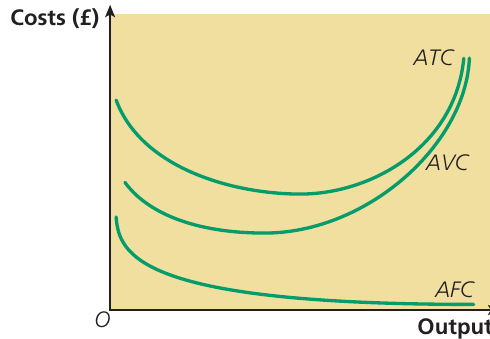
This diagram shows the relationship between all three average cost curves. The ATC curve lies above the AVC curve by the amount of the AFC at each output level. As output increases, the gap between ATC and AVC narrows because AFC is falling continuously.
Worked example: calculating costs from given data
Understanding how to calculate costs from data is an essential exam skill. Let's work through an example.
Worked Example: Calculating Total Cost from Average Cost Data
Question: A firm's average variable costs and average fixed costs are shown in the graph below. What is the total cost of producing 4 units?
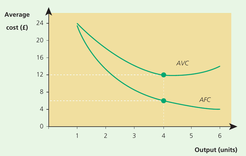
Solution:
To find total cost at 4 units of output, we need to:
Step 1: Find the ATC by adding AFC and AVC at 4 units
- At 4 units: and
- Therefore:
Step 2: Calculate total cost by multiplying ATC by output
The answer is £72.
Exam tip: When calculating costs from graphs, always read values carefully from the axes. Make sure you're clear whether you're looking at average or total costs, as this affects your calculation method.
Bringing together the various short-run cost curves
Understanding how different cost curves relate to each other is crucial for economic analysis.
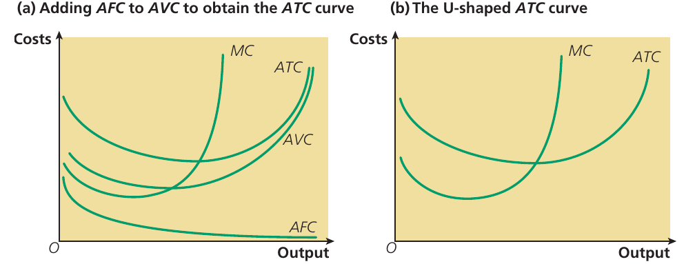
The left panel (a) demonstrates how the ATC curve is formed by adding the AFC and AVC curves vertically at each output level. The marginal cost (MC) curve cuts through both the AVC and ATC curves at their lowest points. This reflects an important mathematical relationship between marginal and average values.
The right panel (b) shows the simplified diagram commonly used in exams. This focuses on the U-shaped ATC curve and the MC curve, which intersects the ATC at its minimum point. This simplified version is often sufficient for analysis.
Key relationships to remember:
- When MC is below ATC, average total cost is falling
- When MC is above ATC, average total cost is rising
- MC intersects ATC at the minimum point of the ATC curve
- The same relationship exists between MC and AVC
This mathematical relationship holds for any marginal and average values, not just costs.
Study tip: Practice sketching these curves and their relationships. Being able to draw accurate cost curve diagrams quickly will help you in exam situations where you need to illustrate your analysis.
How factor prices and productivity affect costs and choice of factor inputs
Factor prices and productivity play a crucial role in determining how firms organise production and which methods they choose.
Understanding factor prices and productivity
Factor prices are the costs firms pay for hiring different factors of production. The main factor prices are:
- Wages and salaries: the reward for hiring labour
- Interest: the reward for hiring capital
Productivity measures output per unit of input:
- Labour productivity: output per worker
- Capital productivity: output per unit of capital employed
The firm's objective: profit maximisation through cost minimisation
Firms generally aim to maximise profit. To achieve this, they must produce their chosen level of output at the lowest possible cost. This requires employing the optimal factor combination that minimises production costs.
When making this decision, firms must consider both factor prices and productivity levels together.
How factor prices influence production methods
If wage levels are low but the price of capital is high, then labour becomes more attractive to employ than capital (assuming we ignore productivity differences for now). In this scenario, a firm should use a labour-intensive method of production, employing many workers but little capital.
Conversely, if labour is expensive but capital is cheap, cost minimisation requires a capital-intensive method of production, using lots of capital but little labour.
The role of productivity
The decision becomes more complex when we consider productivity differences. If wage levels are low but labour productivity is also low, a capital-intensive method might still be preferable, provided the high price of capital is more than offset by high capital productivity.
Real-world example: the UK car industry
Capital-intensive production often comes with high wage rates, though relatively few workers are employed. However, when consumers demand more output from capital-intensive firms, employment of labour also increases.
Case Study: Japanese Car Manufacturers in the UK
Companies such as Nissan and Toyota have demonstrated how capital-intensive production can benefit workers in the UK car industry. These firms employ robots rather than workers to produce car parts. The greater use of robotised machinery has enabled both wage rates and employment levels to rise in the UK car industry, showing how capital-intensive production can benefit workers when demand for output increases.
Key insight: The choice between labour-intensive and capital-intensive production depends on the relative factor prices and productivities, not absolute values. Firms must compare the cost per unit of output for different production methods.
A firm cannot decide simply by looking at wages alone or capital costs alone. The decision requires comparing:
- Wage rate ÷ Labour productivity versus Interest rate ÷ Capital productivity
Remember!
Key Points to Remember:
-
Fixed costs don't change with output in the short run, while variable costs do change with output levels
-
The AFC curve always slopes downwards because fixed costs are spread over more units as output increases (spreading of overheads)
-
The ATC curve is U-shaped and is formed by adding AFC and AVC at each output level
-
Marginal cost (MC) intersects both AVC and ATC at their minimum points
-
Firms choose production methods based on both factor prices and productivity levels to minimise costs and maximise profit