Marginal, Average, and Total Revenue (AQA A-Level Economics): Revision Notes
Marginal, Average, and Total Revenue
Revenue represents the money that a business earns from selling its goods or services. Understanding the different types of revenue and how they relate to each other is essential for analysing firm behaviour in different market structures.
Understanding revenue concepts
When firms sell their output, they generate revenue. There are three key ways to measure this revenue, each providing different insights into a firm's sales performance.
Total revenue (TR) represents all the money a firm receives from selling its entire output of a product. It is calculated by multiplying the price per unit by the quantity sold.
Average revenue (AR) shows the revenue earned per unit of output sold. It is calculated using the formula:
where TR is total revenue and Q is the quantity of output.
Marginal revenue (MR) measures the additional revenue generated from selling one more unit of output. It is calculated as:
where Δ (delta) represents the change in total revenue and the change in quantity.
The delta symbol (Δ) is used in mathematics to indicate a change in value. The word "marginal" specifically refers to the change in a variable when one more unit is produced or sold.
Average revenue and the firm's demand curve
For any firm, the demand curve it faces is identical to its average revenue curve. This is because at each level of sales, the average revenue the firm earns equals the price charged. When the price charged is the same for all units of output sold, the demand curve and the AR curve are the same line.
Worked Example: A Retailer's Demand for Microwave Ovens
Consider a retailer of electrical goods facing demand for microwave ovens in a particular week:
Scenario 1: Price set at $500
- Quantity demanded: 20 ovens
- Total revenue: $10,000
- Average revenue per oven: $500
Scenario 2: Price reduced to $300
- Quantity demanded: 60 ovens
- Total revenue: $18,000
- Average revenue per oven: $300
At each level of sales, the average revenue equals the price charged, demonstrating that the demand curve facing the firm is also its average revenue (AR) curve.
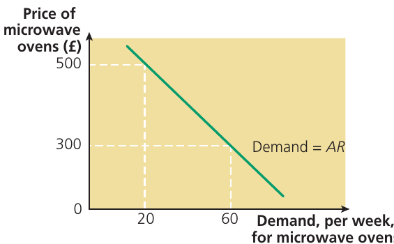
The key point is that at each level of sales, the average revenue the retailer earns equals the price charged. Therefore, the demand curve facing the firm is also its average revenue (AR) curve.
The relationship between average and marginal revenue
When marginal and average values are plotted from the same data set, they always display a consistent mathematical relationship:
Critical Mathematical Relationship:
- When the marginal is greater than the average, the average rises
- When the marginal is less than the average, the average falls
- When the marginal equals the average, the average is constant (neither rising nor falling)
This relationship applies to all marginal and average values, including marginal and average returns, marginal and average costs, and marginal and average revenue.
Understanding this relationship helps explain the shapes of revenue curves in different market structures.
The specific shape of a firm's revenue curves depends on the competitiveness of the market structure in which it operates. The two most important market structures for understanding revenue curves are perfect competition and monopoly.
Revenue in perfect competition
A perfectly competitive market must satisfy six key conditions:
- A very large number of buyers and sellers
- All buyers and sellers possess perfect information about market conditions
- Consumers can buy as much as they wish and firms can sell as much as they wish at the ruling market price
- No individual consumer or supplier can affect the ruling market price through their own actions
- The product is identical, uniform or homogeneous
- There are no barriers to entry into, or exit from, the market in the long run
In perfect competition, each individual firm is a price-taker. This means the firm is so small relative to the market that it must accept the ruling market price. If the firm raises its price above the market price, it loses all its sales because customers desert it to buy identical products from other firms at the lower market price. Conversely, there is no point selling below the ruling market price because the firm can already sell any quantity it wants at the market price.
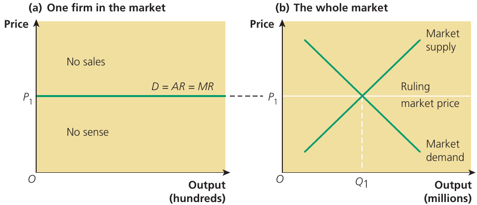
The diagram shows two panels: panel (a) depicts an individual firm facing a horizontal demand curve at price P₁, while panel (b) shows the whole market where supply and demand intersect to determine the equilibrium price P₁ and quantity Q₁.
For a firm in perfect competition, the ruling market price is both the firm's average revenue curve and its marginal revenue curve. If each unit of the good is sold at a price of $1 (average revenue), selling an extra unit always increases total revenue by $1 (marginal revenue). The horizontal price line is also the perfectly elastic demand curve for the firm's output.
In summary, for a perfectly competitive firm: D = AR = MR. The demand curve, average revenue curve, and marginal revenue curve are all the same horizontal line at the market price.
Revenue in monopoly
The demand curve facing a perfectly competitive firm is horizontal at the ruling market price and represents the firm's AR curve. By contrast, the demand curve for a monopolist's output is the market demand curve, which slopes downwards. This is the monopolist's AR curve, but it is not the monopolist's MR curve.
When a firm faces a downward-sloping demand curve, it becomes a price-maker. This means it possesses market power to set the price at which it sells the product. However, a firm cannot be both a price-maker and a quantity-setter at the same time.
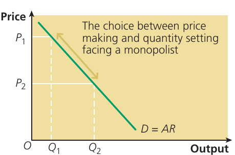
If the monopolist chooses to set the price at P₁, the demand curve dictates the maximum output that can be sold at this price (Q₁). Alternatively, if the monopolist chooses to set the quantity at Q₂, the demand curve shows that the maximum price at which this quantity can be sold is P₂.
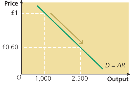
The downward-sloping market demand curve facing the monopolist is the firm's average revenue (AR) curve. At a price of $1, 1,000 units are demanded, giving total revenue of $1,000 and average revenue of $1. At $0.60, 2,500 units are demanded, giving total revenue of $1,500 and average revenue of $0.60.
Marginal revenue and average revenue are not the same in monopoly.
To understand why, remember that when the marginal value of a variable is less than the average value, the average value falls. Because the market demand curve (or average revenue curve) falls as output increases, the monopolist's marginal revenue curve must be below its average revenue curve.
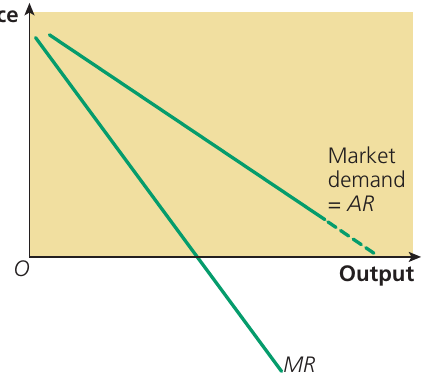
This diagram illustrates how the MR curve lies below the AR curve and is twice as steep when the AR curve is a straight line.
Explaining the relationship between AR and MR in monopoly
When a monopolist increases sales, two opposing effects occur:
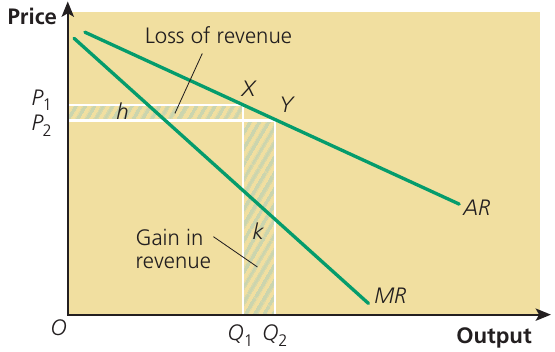
The monopolist initially charges price P₁ and sells output Q₁. To increase sales to Q₂, the downward-sloping AR curve forces the monopolist to reduce the selling price to P₂. This reduces the price at which all units of output are sold.
Total revenue increases by the area k (the gain in revenue from selling extra units). However, total revenue decreases by area h (the loss of revenue from selling all previous units at a lower price). Marginal revenue, which is the revenue gain minus the revenue loss, must be less than price or average revenue.
Areas h and k respectively show the revenue loss and the revenue gain. The extra unit sold multiplied by price P₂ represents the revenue gain, while in order to sell more, the price has to be reduced for all units of output, not just the extra unit sold.
Price elasticity and revenue
The relationship between price elasticity of demand and revenue is important for understanding monopoly behaviour. Along a straight-line demand curve, elasticity varies.
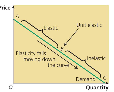
In the upper portion of the demand curve, demand is elastic. At the midpoint, demand is unit elastic. In the lower portion, demand is inelastic. Elasticity falls when moving down the curve.
In perfect competition, the demand curve for an individual firm is perfectly elastic (horizontal). This is because the output of every other firm in the market is a perfect substitute for the firm's own product. If the firm tries to raise its price above the ruling market price, it loses all its customers to competitors.
In monopoly, by contrast, the demand curve is downward-sloping. Because the demand curve is a straight line, price elasticity of demand falls moving down the curve. Demand for the monopolist's output is elastic in the top half of the curve, falling to unit elastic at the midpoint.
The relationship between marginal revenue and total revenue
Marginal revenue measures the change in total revenue that results from an increase in the quantity of goods sold. It indicates how much revenue increases for selling an additional unit.
Marginal revenue is shown by the slope of the total revenue curve:
- Increasing marginal revenue is shown by the total revenue curve becoming steeper
- Falling marginal revenue is shown by the total revenue curve becoming less steep as sales increase
- Constant marginal revenue means that the slope of the total revenue curve is unchanged as sales increase
This illustrates another example of the relationship between marginal and total values of a variable. The relationship between marginal costs and total cost provides a third example of this important mathematical relationship.
Remember!
Key Points to Remember:
- Total revenue is all the money earned from selling total output; average revenue is revenue per unit (TR/Q); marginal revenue is the additional revenue from selling one more unit (ΔTR/ΔQ).
- The demand curve facing a firm is identical to its average revenue curve because price equals average revenue at each level of output.
- In perfect competition, firms are price-takers facing a horizontal demand curve where D = AR = MR.
- In monopoly, firms are price-makers facing a downward-sloping demand curve where the marginal revenue curve lies below the average revenue curve.
- When marginal is greater than average, the average rises; when marginal is less than average, the average falls; when marginal equals average, the average stays constant.